
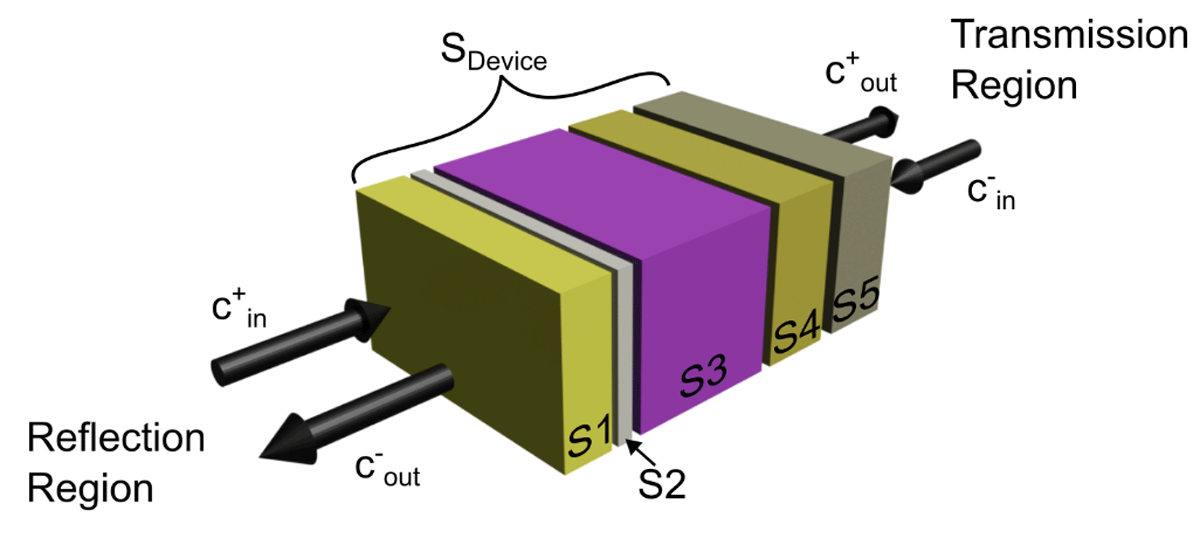
Figure 1
Visual representation of the layer cascading process in the SMM. The schematic is defined by three main regions. First, the reflection region above the stack, assuming incident light comes from this side, where the front surrounding medium and incident light properties are defined. Second, there is the transmission region, right-side, that defines the rear surrounding medium. Here, c-in is 0 (no rear incident light). The defined object layers are in between these regions, represented by the S1–S5 scattering matrices. The composite scattering matrix for the full layer stack is termed SDevice.
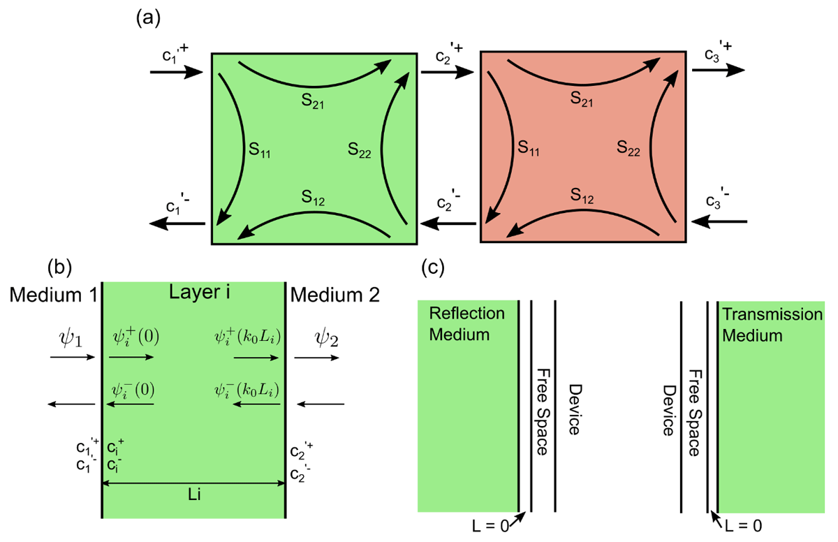
Figure 2
Schematic representation of different steps in the formulation of the scattering matrix method. (a) Schematic showing the scattering matrix elements, S11, S12, S21 and S22, as well as the mode coefficients, c, that describe the internal interaction of light with a specific layer. The schematic also shows how the mode coefficients can be used to connect different layers. (b) Schematic showing the solutions to the matrix-wave equation, where ci+/- are the mode coefficients for layer i and ϕi the solutions for a particular layer. (c) Schematic defining the scattering matrices for the reflection (left) and transmission (right) regions. Here, we defined the medium for the scattering matrix to be vacuum.
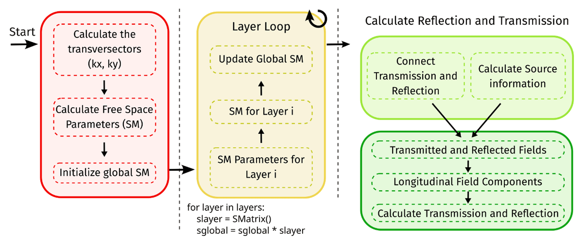
Figure 3
Pseudo-code schematic indicating the three main implementation sections for the scattering matrix (SM) method code. In red, there is the initialization section, where the incident light information is determined and the global scattering matrix (SGlobal) is initialized; the second section is the layer loop, where the scattering matrix for each layer is determined and the global scattering is thus updated; the last section is the finalization step, where the transmission and reflection region information is added followed by the determination of the transmission and reflection.
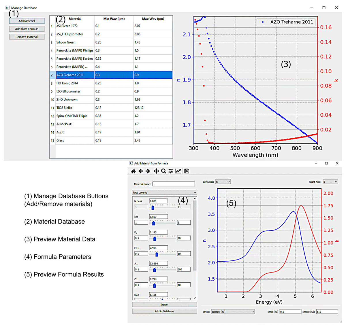
Figure 4
Graphical visualization of the database of experimentally obtained refractive index spectra (top), as well as of the applet to add modelled spectra (bottom) windows. The database window is divided into 3 main panels; the manage database buttons (1), the materials database (2) and the graph to preview the refractive index data (3). The add formula window is divided into 2 main panels; the model parameters control (4) and the graph to preview the resulting refractive index with the current settings (5).
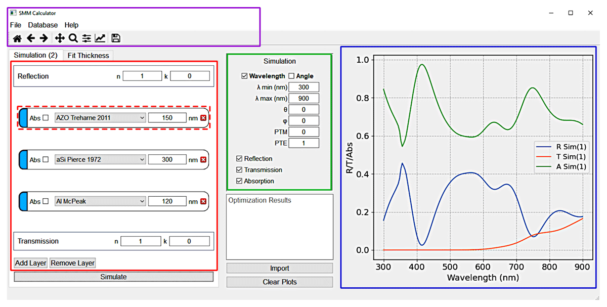
Figure 5
Main interface panels of the SCATMM program highlighted in a different colour. The purple panel is the main menu, including access to the database, help and the session-stored simulations. The red panel is the core element of the interface where the layers and surrounding materials are defined. The green panel is where the simulation configuration is defined. The blue panel is the preview region, where the simulated results are shown.
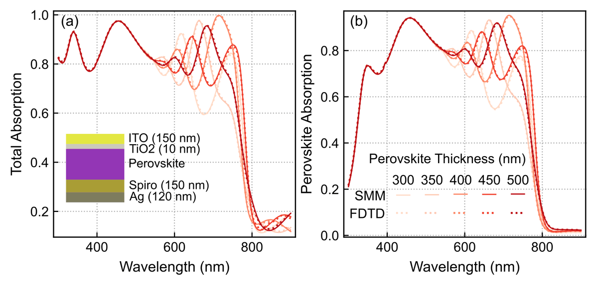
Figure 6
Comparison of computed absorption spectra between the FDTD (dotted lines) and SMM (full lines) methods, considering normal light incidence on a perovskite solar cell (PSC) with changing perovskite thickness from 300 to 500 nm. (a) Total absorption in the PSC multilayer structure (depicted in inset); (b) Useful absorption only within the perovskite layer that generates photocurrent.
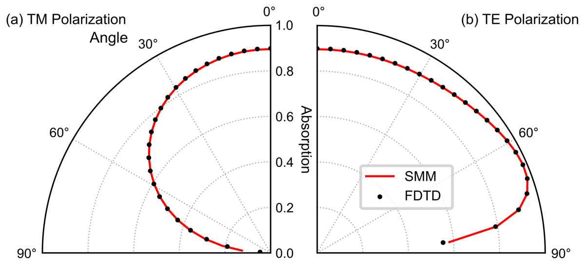
Figure 7
Comparison of angular absorption profiles between the SMM and the FDTD method, considering light incident at different angles on the same PSC structure of Figure 4 with 500 nm perovskite thickness. The dotted lines indicate the FDTD results and the full red lines the SMM results. (a) Results for the transverse magnetic (TM) polarization; (b) results for the transverse electric polarization (TE).
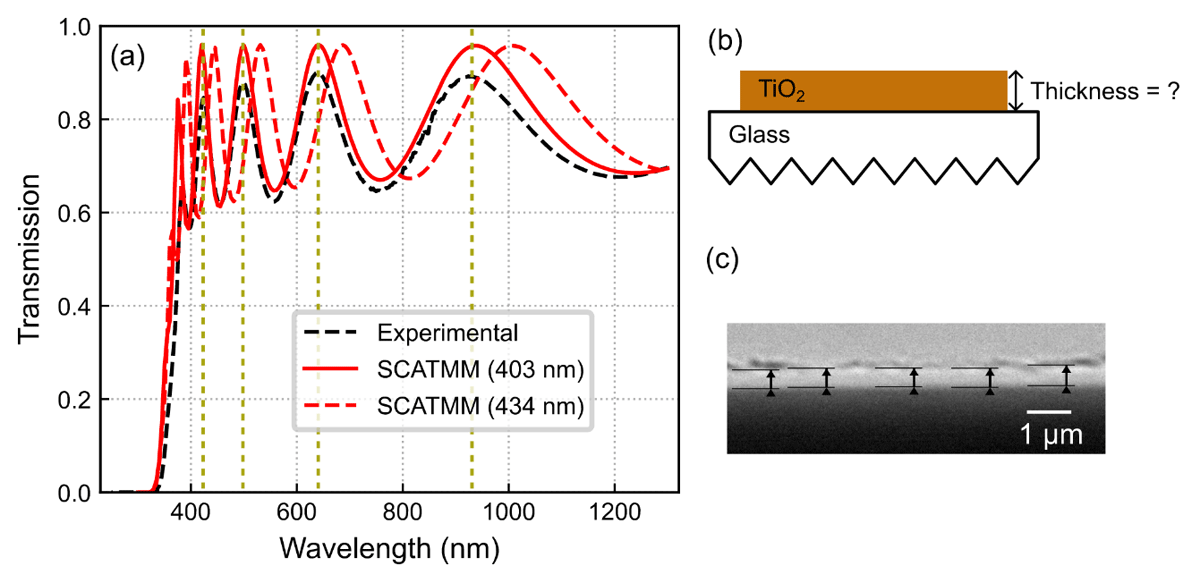
Figure 8
(a) Comparison between the spectra of the experimental measured transmission via spectrophotometry (black dashed lines) and the SCATMM transmission for both the best peak-matching thickness of 403 nm (full red line), and a thickness equal to the average profilometry measurement of 434 nm (dashed red line). (b) Schematic of the SCATMM simulation configuration, namely the TiO2 top layer and the glass substrate. The corrugated glass bottom indicates that it was defined as an infinite layer. (c) Cross-sectional SEM image of the TiO2 layer. The arrows indicate the different places measured to determine the average thickness.