

Figure 1
Flowchart of the typical workflow of generating status and trend estimates using bbsBayes for any species of North American bird covered by the North American Breeding Bird Survey.
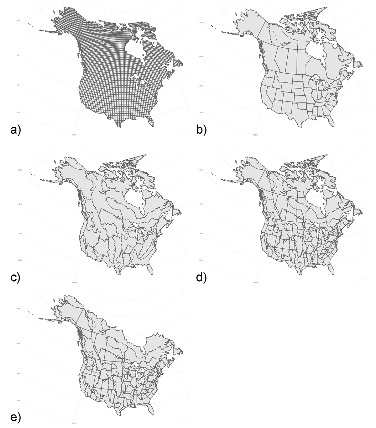
Figure 2
Maps of the 5 stratification options offered by bbsBayes. A user can specify to stratify by degree blocks (a), state (b), Bird Conservation Region (BCR; c), BCR × state (USGS method; d), or BCR × state (CWS method; e).
Table 1
Comparison of the 4 models provided by bbsBayes.
| MODEL | TEMPORAL PARAMETERS | DESCRIPTION | REFERENCE |
|---|---|---|---|
| Slope model = “slope” | Random-effect log-linear slopes (overall long-term rate of population change) with random year-effect deviations (yearly fluctuations around the overall long-term slope). | Based on the model used by the CWS and USGS since 2011, but with slopes and intercepts fit as random effects, so that slopes and intercepts for data-sparse strata are shrunk towards the survey-wide means. | [16] |
| First-difference model = “firstdiff” | Year-effects follow a random walk, where for each stratum, the differences between year-t and year-t-1 is a zero-mean normal distribution with an estimated variance. | Based on the first-difference model described in Link and Sauer 2020. [33] The year-effects are shrunk towards the value in the previous year, so that the long-term trajectory is relatively flexible (e.g., can follow cyclical population patterns well) but annual fluctuations are dampened. | [17] |
| GAM model = “gam” | Year-effects follow a penalized thin-plate spline (i.e., a GAM smooth), with a number of knots chosen by the user. The parameters linking the basis function to the yearly values are estimated as random effects, centred on a survey-wide mean, so that the shape of the trajectory in a data-sparse stratum is shrunk towards a survey-wide mean trajectory. | GAM basis structure based on Crainiceanu et al. 2005. [24] For a number of knots, similar to the defaults (0.25 * number of years), the estimated trajectories are relatively smooth in the short-term (i.e., show no annual fluctuations) but are quite flexible over the long- and medium-term (e.g., population cycles on a 3-10 year period and change points in medium-term trends are modelled well). | [10] |
| GAMYE model = “gamye” | Combines the GAM components of the above model with the random year-effects of the slope model. | Trajectories are quite flexible over the long- and medium-term (e.g., population cycles on a 3–10 year period and change points in medium-term trends are modelled well), and include yearly fluctuations around the smoothed trajectory. | [10] |
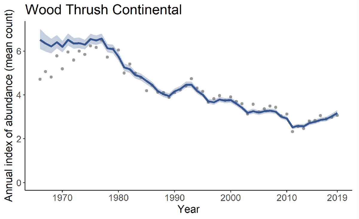
Figure 3
Plot of continental annual index of abundance for Wood Thrush from 1966 to 2019 with 95% credible band and observed means (grey dots). This plot was generated using the plot_indices() function.
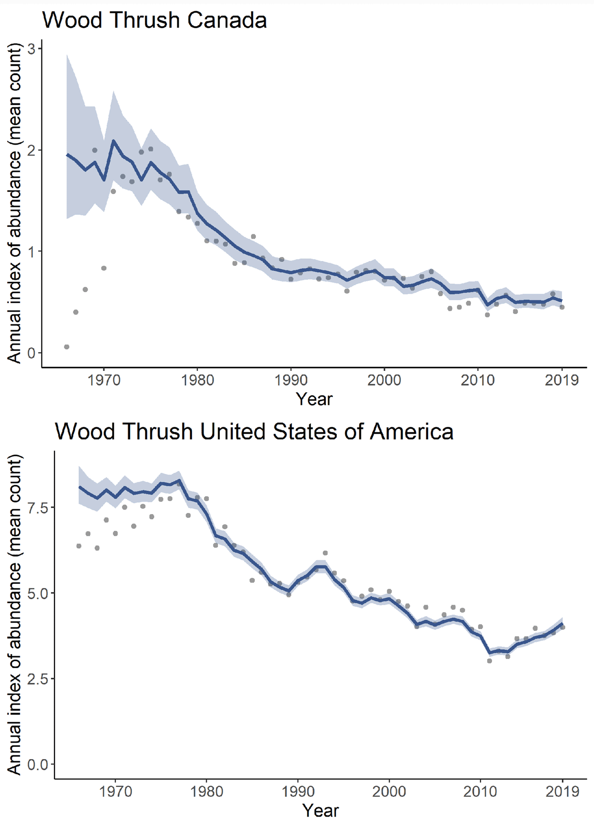
Figure 4
Plots of national annual indices of abundance for Wood Thrush from 1966 to 2019 for Canada and USA. These plots were generated using the plot_indices() function.
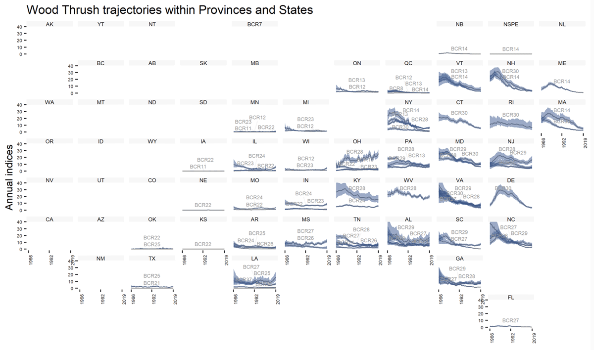
Figure 5
Geofacet plot of Wood Thrush trajectories for each province, state, and territory, created using the plot_geofacet() function. Each line within a state represents the trend (and 95% credible interval) for each BCR within the state.
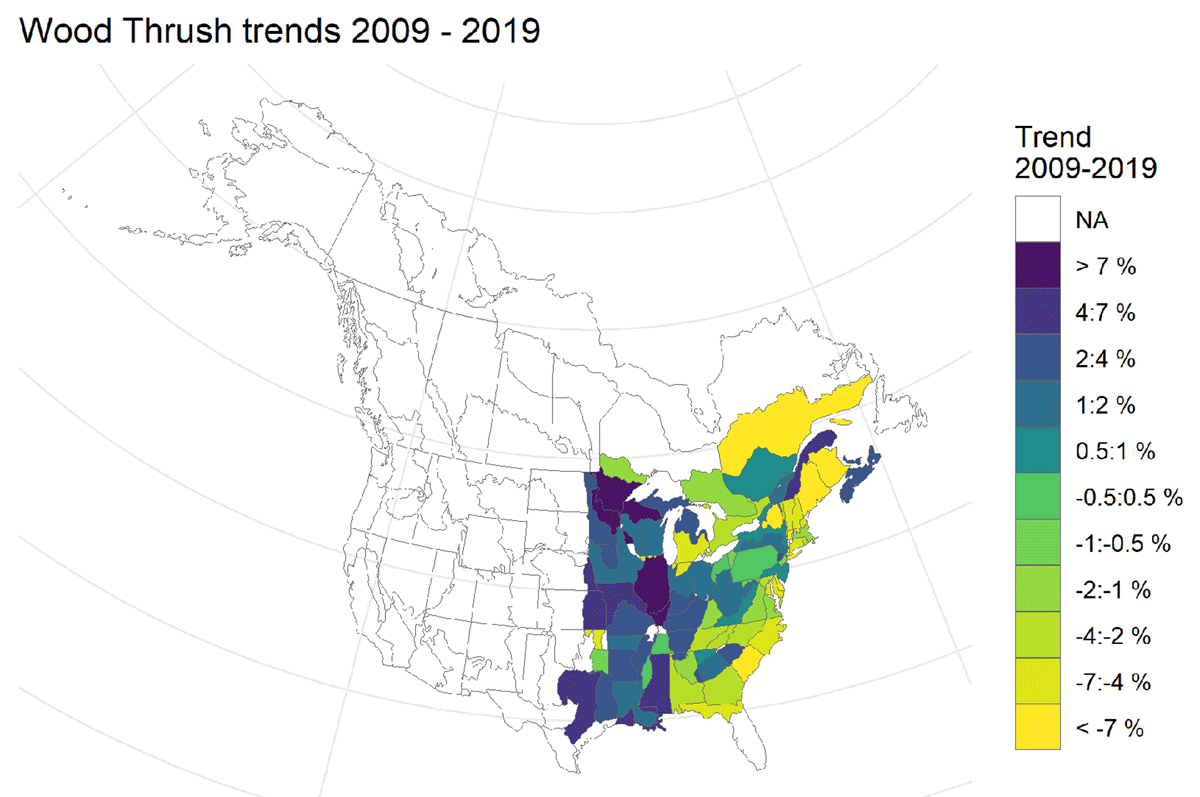
Figure 6
Heat map of Wood Thrush trends for each stratum for the 10-year period between 2009 and 2019. This map was generated using the generate_map() function.
Table 2
Percent change (and 95% credible interval) and probability of changes for the continent-wide trend, national trends, and stratum-level trends for select strata for Wood Thrush between 2009–2019. Based on the function that was run, these probabilities show the probability of the Wood Thrush population decreasing by 0%, 50%, and 100% in each of the geographical regions.
| REGION | PERCENT CHANGE [LOWER LIMIT, UPPER LIMIT] | PROBABILITY OF DECREASING BY 0% | PROBABILITY OF DECREASING BY 50% | PROBABILITY OF DECREASING BY 100% |
|---|---|---|---|---|
| Continental | +5.23% [+0.26%,+10.6%] | 0.02 | 0.00 | 0.00 |
| Canada | –16.4% [–30.7%,+0.56%] | 0.97 | 0.00 | 0.00 |
| United States | +6.45% [–1.30%,+12.0%] | 0.01 | 0.00 | 0.00 |
| US-SC-27 | –74.5% [–84.2%,–57.7%] | 1.00 | 1.00 | 0.00 |
| CA-ON-12 | –16.4% [–39.5%,+14.6%] | 0.87 | 0.00 | 0.00 |
| CA-QC-12 | +6.71% [–36.1%,+80.2%] | 0.40 | 0.00 | 0.00 |
| US-LA-25 | +13.6% [–23.3%,+66.2%] | 0.26 | 0.00 | 0.00 |