
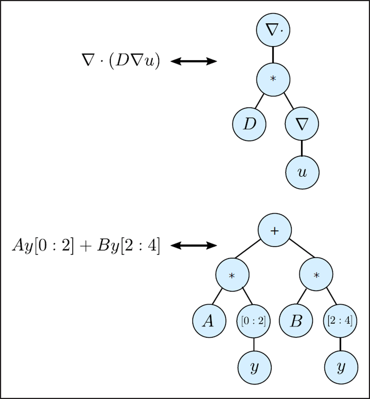
Figure 1
Models are encoded and passed down the pipeline using a symbolic expression tree data-structure. Leafs in the tree represent parameters, variables, matrices etc., while internal nodes represent either basic operators such multiplication or division, or continuous operators such as divergence or gradients.
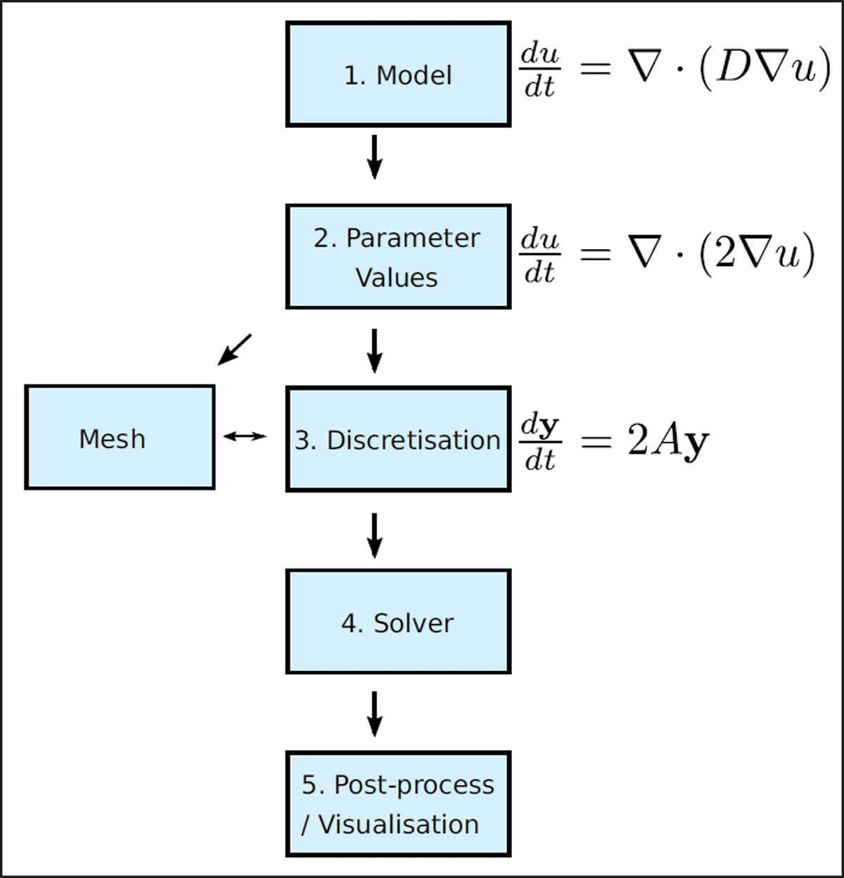
Figure 2
PyBaMM is designed around a pipeline approach. Models are initially defined using mathematical expressions encoded as expression trees. These models are then passed to a class which sets the parameters of the model, before being discretised into linear algebra expressions, and finally solved using a time-stepping class.
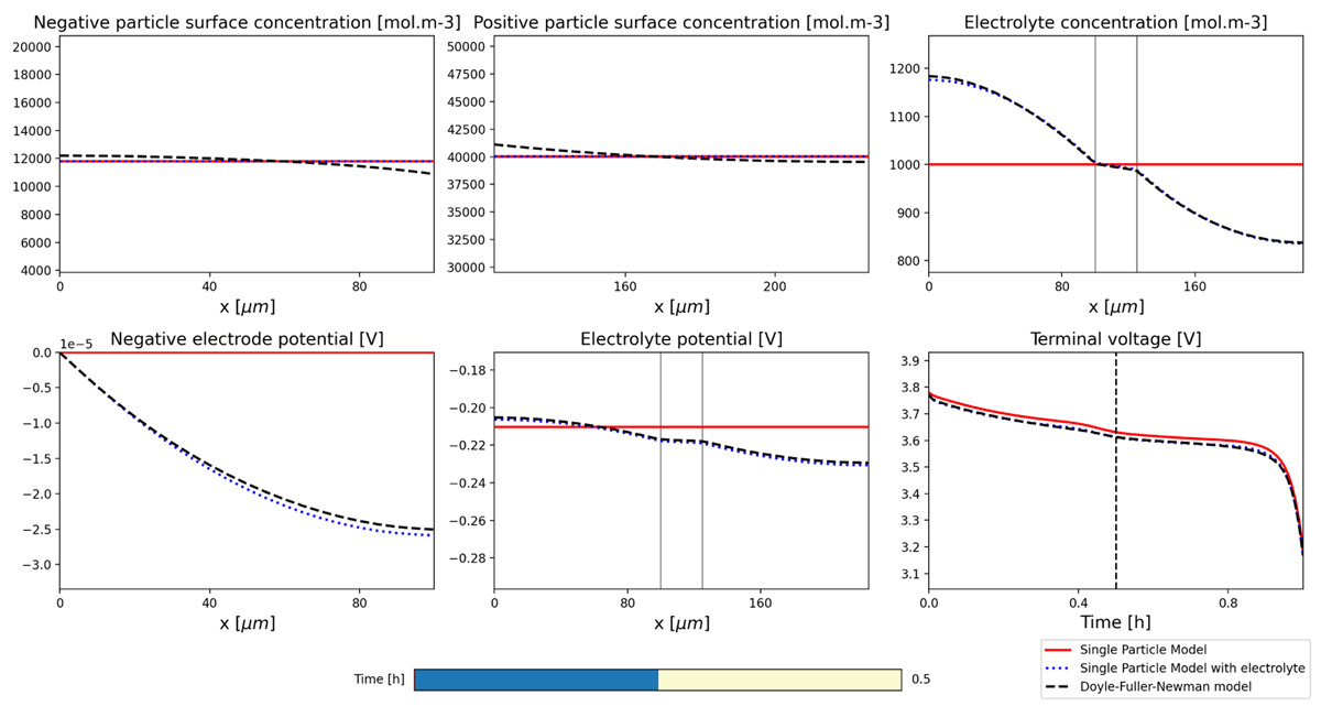
Figure 3
Interactive visualisation of solutions. The user can select the time at which to view the output using the time-slider bar at the bottom. This interactive plot is automatically generated by providing a list of model solutions and output variables.
Listing 1
Running a simulation in PyBaMM.
| 1 | import pybamm |
| 2 | # Doyle-Fuller-Newman model |
| 3 | model = pybamm.lithium_ion.DFN() |
| 4 | sim = pybamm.Simulation(model) |
| 5 | sim.solve([0, 3600]) # solve for 1 hour |
| 6 | sim.plot() |
Listing 2
Running an experiment in PyBaMM.
| 1 | import pybamm |
| 2 | experiment = pybamm.Experiment( |
| 3 | [ |
| 4 | ″Discharge at C/10 for 10 hours or until 3.3 V″, |
| 5 | ″Rest for 1 hour″, |
| 6 | ″Charge at 1 A until 4.1 V″, |
| 7 | ″Hold at 4.1 V until 50 mA″, |
| 8 | ″Rest for 1 hour”, |
| 9 | ] |
| 10 | * 3, |
| 11 | ) |
| 12 | model = pybamm.lithium_ion.DFN() |
| 13 | sim = pybamm.Simulation( |
| 14 | model, |
| 15 | experiment=experiment, |
| 16 | solver=pybamm.CasadiSolver(), |
| 17 | ) |
| 18 | sim.solve() |
| 19 | sim.plot() |
Listing 3
Defining a model in PyBaMM.
| 1 | # 1. Initialise model |
| 2 | model = pybamm.BaseModel() |
| 3 | |
| 4 | # 2. Define parameters and variables |
| 5 | c = pybamm.Variable(″c″, domain=″unit line″) |
| 6 | k = pybamm.Parameter(″Diffusion parameter″) |
| 7 | |
| 8 | # 3. State governing equations |
| 9 | D = k * (1 + c) |
| 10 | dcdt = pybamm.div(D * pybamm.grad(c)) |
| 11 | model.rhs = {c: dcdt} |
| 12 | |
| 13 | # 4. State boundary conditions |
| 14 | D_right = pybamm.BoundaryValue(D, ″right″) |
| 15 | model.boundary_conditions = { |
| 16 | c: { |
| 17 | ″left″: (1, ″Dirichlet″), |
| 18 | ″right″: (1/D_right, ″Neumann″) |
| 19 | } |
| 20 | } |
| 21 | |
| 22 | # 5. State initial conditions |
| 23 | x = pybamm.SpatialVariable(″x″, domain=″unit line″) |
| 24 | model.initial_conditions = {c: x + 1} |