
1 Overview
Repository location The data is released on Zenodo: https://doi.org/10.5281/zenodo.19497434.
1.1 Context
Source
At the end of the 19th century, the five-feet to the mile map of London by the Ordnance Survey (OS) depicted the city and suburbia in high detail, when it was the largest city in the world, with an estimated population of 5.6 million (Bartholomew, 1899). As such, the map was the first comprehensive large-scale representation of the Greater London area. The initial survey of the city centre was carried out between 1848 and 1850 for the Metropolitan Commissioners of Sewers, following the Public Health Act of 1848 (Hyde, 1975). The principal aim was to create a sanitary tool to organise and plan the development of the sewer network, and to regulate activities that could pose a sanitary threat, such as slaughtering and tanning. The so-called “Skeleton Survey” was carried out by OS engineers, at the scale of five-feet to the mile (1:1,056) (Hyde, 1975). The full engraving and publication of this map at that scale was, however, never finished (Oliver, 2013). Between 1863 and 1874, a second survey was carried out. The sheets, engraved at a scale of 1:1,056 and published between 1867 and 1876, included much fuller topographic details (Oliver, 2013). The 1890s OS map used here was a revision of that second map, encompassing not only the city centre but also the broader metropolitan area, corresponding to a land surface twice as large. The revision and complementary survey were undertaken between 1891 and 1895; the plans were published between 1893 and 1896 (Oliver, 2013). The 1891–96 1:1,056 mapping of London was printed by the OS office in Southampton, using a photozincographic reproduction process. Each physical sheet is about 74 × 105 cm, with a map neat-line extent of 61 × 92 cm.
Digital object
The plans were digitised by the National Library of Scotland in 2013, at a resolution of 400 ppi. The manual grid georeferencing was carried out by the National Library of Scotland, with funding from David Rumsey. The released digital object comprises 753 georeferenced map sheets. Six sheets appear to be missing (National Library of Scotland, 2013; Oliver, 2013)1. Figure 1 shows the resulting building footprint layer.
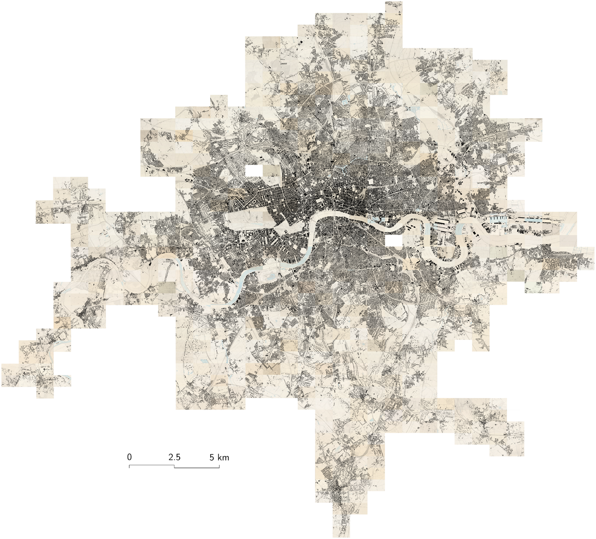
Figure 1
Overview of the London building footprints layer, overlaid on the georeferenced 1890s OS map. The building footprints are coloured in black.
Previous work
Although the size of this corpus makes manual vectorisation prohibitive, the development in recent years of neural models for recognising geographic information in historical maps offers a plausible avenue for retrieving building footprints. Several pioneering works have indeed addressed the detection of footprints in historical maps (Heitzler & Hurni, 2020; Herold & Hecht, 2018; Oliveira et al., 2019). Litvine et al. (2024) employed similar methods to extract built-up areas from early historical maps, including 1746, 1799, and 1830 maps of London. For large-scale plans—cadastral or parcel-based, such as the one addressed in this paper—the vectorisation of individual footprints is particularly sensitive to the detection of boundaries, on which the segregation of objects relies (Chazalon et al., 2021; Chen et al., 2021, 2024; Göderle et al., 2024; Petitpierre & Guhennec, 2023). To address this issue, we pair a generic segmentation model (Petitpierre, 2026) pretrained on historical OS maps of London with a specialist boundary-detection model (Petitpierre et al., 2024), and follow the vectorisation procedure of Vaienti et al. (2023).
Collaboration context
The digital layer of building footprints was created in the context of an international collaboration between EPFL, the Swiss Federal Institute of Technology in Lausanne, the Alan Turing Institute, the University of Cambridge, the Colouring Cities Research Programme, the Leibniz Institute of Ecological Urban and Regional Development (IOER), the National Library of Scotland, Lancaster University, and the University of Bristol. A collective annotation workshop was organised in Lausanne, Switzerland, 25-26 April 20242. The workshop involved over 20 participants from the above-mentioned partners, as well as invited presenters from ETH Zurich, the University of Bristol, the University of Jena, and the Bibliothèque nationale de France (BnF).
2 Method
2.1 Steps
The dataset results from an entirely automatic extraction process, based on deep semantic segmentation technologies.
First, a subset of 262 image patches, of size 768 × 768 px, extracted from the original scanned map, were manually labelled with the Computer Vision Annotation Tool (CVAT) (Intel, 2020). 62 samples were used for validation, 20 for testing, and 180 samples were used for training the segmentation model, corresponding to approximately one-tenth of one per cent of the entire map. The annotation included two separate classes (cf. Figure 2). The first class corresponds to regular building footprints. The second class addresses a specific case: namely, compound building geometries. This class includes public buildings with interior ground floor details, such as churches, chapels, railway stations, and covered markets, as well as passageways and glass-roofed buildings. The distinction was motivated more by cartographic visualisation and processing requirements than by geographic ontology. Indeed, churches and other public buildings are usually depicted with interior architectural details of the ground floor, such as inner walls, rooms and stairs. The segmentation model tends to detect these subdivisions, resulting in multiple polygons instead of building-level geometries. The compound building class makes it possible to merge the subparts in a post-processing step. Other edge cases addressed by this class include covered passageways and archways, depicted by a cross marking the passageway, and glass-roofed buildings, filled with a cross-hatched (or diamond-shaped) grid texture, both of which present the same challenge. The compound building class was introduced after the initial tests specifically to mitigate oversegmentation issues.
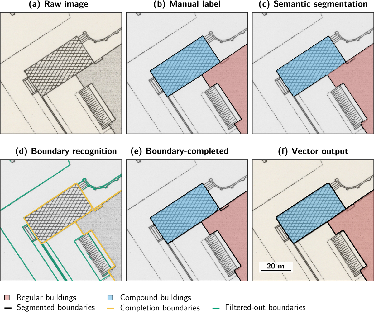
Figure 2
Overview of the footprint extraction method. (a) Initial map image; (b) Manual label of semantic classes (ground-truth); (c) Result of the London segmentation model; (d) Result of the specialist boundary-detection model, with selected boundaries in radius r ≤ 10 of building surfaces coloured in yellow and excluded ones in green; (e) Combined segmentation mask after boundary completion; (f) Final vector output.
Whereas collaborative annotation on CVAT results in vector-format data, semantic segmentation models require pixel-level raster labels. Vector geometries were thus rasterised in a subsequent step. Upon rasterisation, a third class was created, namely building boundaries, corresponding to the contours of annotated vector objects. Practically, boundaries correspond to raster lines with a fixed width of three pixels. This class is instrumental in retrieving building-level footprints, since semantic segmentation, unlike panoptic or instance segmentation, does not otherwise segregate adjacent objects.
Semantic segmentation
The aim of semantic segmentation models is to assign a semantic class (regular or compound building, boundary) to each pixel in a raster image (in this case, map sheets). We rely on OpenMMLab’s (OpenMMLab, 2022) implementation of the Mask2Former (Cheng et al., 2022) architecture. The model was trained for 48,000 iterations3. Optimisation relied on cross-entropy loss, a batch size of one, and the AdamW optimiser with a polynomial scheduler and a learning rate starting at 8⋅10–6. Ultimately, we obtained a mean class intersection-over-union (IoU) of 84.2% (regular buildings 96.3%, compound buildings 82.6%, boundaries 73.7%). Inference is performed hierarchically, following the strategy described by Petitpierre (2026).
Boundaries completion
Despite the good performance in classifying and recognising buildings, the ability to vectorise geometries accurately largely hinges on the model’s ability to generate completely bounded components. This requirement is particularly sensitive to false negative errors, e.g., short interruptions in the object boundary, as visible in Figure 2. To address this challenge, a separate, specialist segmentation model is trained for boundary recognition on a distinct corpus, corresponding to diverse parcel plans (Petitpierre et al., 2024). This operational choice is also justified by the contrast between the two tasks: the classification of regular and compound buildings on the one hand, and the detection of thin, filamentary boundaries on the other hand. The predictions of the specialist model are then merged with those of the generic model. Boundaries outside a radius of 10 pixels from the predicted building surfaces are then filtered out. The vectorisation process follows the procedure described by Vaienti et al. (2023). Overall, the automated vectorisation resulted in the extraction of 1,300,831 footprints (1,241,221 regular and 59,610 compound buildings).
2.2 Quality control
The quality of the extracted vector footprints is verified based on the manual correction of multiple distinct, contiguous areas, distributed at regular intervals across the entire map, corresponding to 4,798 polygons. The use of two independent boundary detection models significantly improves building detection recall and precision. The original London model only achieves a recall of 42.3%, with a precision of 43.0%. The specialist boundary detection model exhibits a higher recall (80.2%), but a similar precision (44.8%). When combined, the two models reach a detection recall of 95.4%, with a precision of 97.8%. The improvement reflects the sensitivity of the vectorisation algorithm to interrupted building boundaries: missing or broken contour segments often cause adjacent footprints to merge or be discarded. By adding specialist contour predictions, the combined model closes many of these breaks while limiting spurious boundaries, improving both recall (e.g., fewer missing buildings) and precision (e.g., fewer merged or oversegmented building footprints) significantly. Overall, we count 4,579 true positives, 101 false positives, and 219 false negatives in the test sample. As visible in Figure 3, smaller footprints tend to be less accurately detected compared to larger ones. Misdetection of larger buildings, however, often tends to be visually more impactful. Other remaining challenges include the disruption caused by sheet borders, as visible in Figure 4.
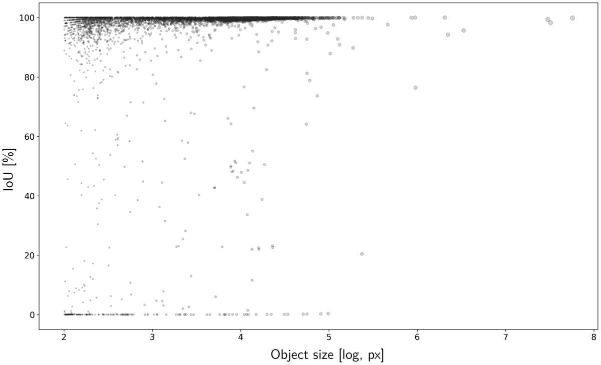
Figure 3
Evaluation of building detection, measured by the IoU, as a function of object size.
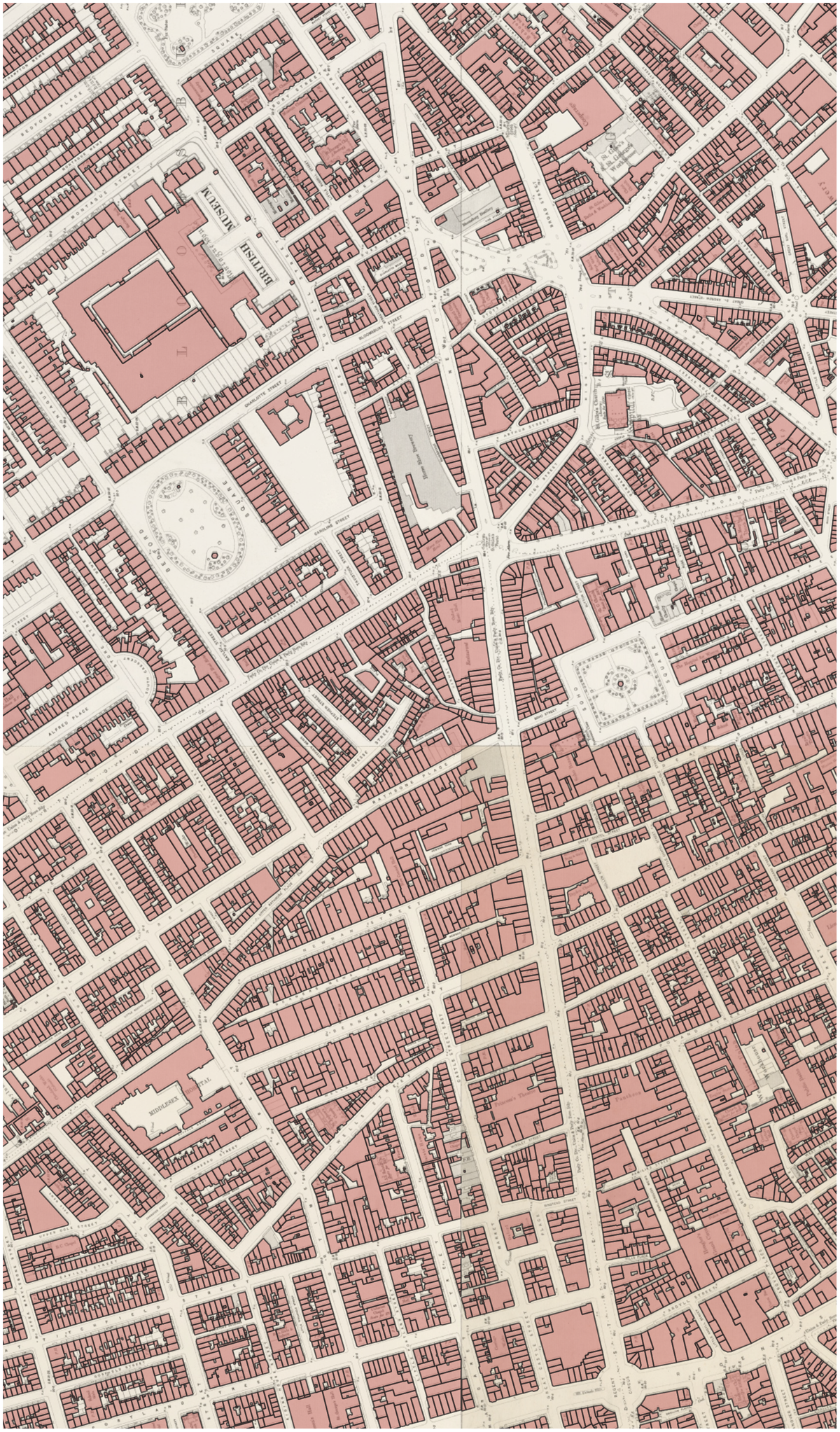
Figure 4
Example of vectorisation result, overlaid on the original georeferenced map layer.
Beyond detection quality, we assess the positional accuracy of the georeferenced footprints by comparing 80 manually validated ground control point pairs between historical buildings and their present-day OpenStreetMap counterparts4. We find a mean displacement of 4.1 m (3.8–4.3 m 95% CI, median 4.0 m, standard deviation 1.1 m), with offsets ranging from 2.1 to 7.9 m. This residual corresponds to the combined effect of the original surveying inaccuracies and the georeferencing error of the digitised sheets.
3 Dataset Description
Repository name
The dataset is hosted on Zenodo and EPFL Infoscience, under the name A Layer of Late Victorian London: The Building Footprints from the 1:1,056 Ordnance Survey Map (1891–1896).
Objects
We publish two distinct versions of the building footprints:
london_buildings_1891-96_raw.gpkg. Raw result of the automatic extraction, corresponding to building footprints after vectorisation and compound building polygon merging.
london_buildings_1891-96_corr_v1.gpkg. Minimally edited version, suitable for downstream studies or visualisation. This initial release version includes minor, partial manual corrections primarily focusing on larger objects, including certain railway stations, monuments, religious edifices, and major warehouses.
Each geometry has an attribute buil_class, taking values in [’regular’,’compound’], that documents the building class and associated processing method. In corr_v1, manually added geometries take the value NULL, while modified/corrected geometries retain their original buil_class. In addition, we release the labelled training and validation data, for reproducibility.
Format names and versions
The data is saved in GeoPackage (.gpkg) format. The coordinate reference system (CRS) is WGS 84 Pseudo-Mercator (EPSG:3857). The use of this Web Mercator projected CRS follows the original CRS in which the historical map sheets were georeferenced.
Creation dates
Original map surveyed 1891–1895, published 1893–1896. Map series digitised and georeferenced in 2013. Vector data created between 2024-04 and 2025-02.
Dataset creators
Remi Petitpierre, EPFL, the Swiss Federal Institute of Technology in Lausanne
Isabella di Lenardo, EPFL
Polly Hudson, University of Cambridge and the Alan Turing Institute (London)
Hendrik Herold, Leibniz Institute of Ecological Urban and Regional Development (IOER, Dresden)
Katherine McDonough, University of Lancaster and the Alan Turing Institute (London)
Robert Hecht, Leibniz Institute of Ecological Urban and Regional Development (IOER, Dresden)
Beatrice Vaienti, EPFL
Christopher Fleet, National Library of Scotland (Edinburgh)
Damien Gomez Donoso, EPFL
Ben Kriesel, EPFL
Language
English.
Licence
Publication date
(2026-07-09).
4 Reuse Potential
The data may be reused, with proper citation, as defined in the CC BY 4.0 licence. Considering the historical significance of the original source, the extensive coverage, and the high spatial granularity, the layer may be of particular interest for research on urban history and related fields, including urban economics, social and economic history, and industrial history. Relevant topics may, for instance, include the study of urban change, persistence, the history of urban planning, working-class housing, or Victorian architecture. The compound building class can also support the study of specific architectures, including monuments, glass-roofed buildings, and covered passageways.
The footprints can also be used as a detailed historical reference layer for London and combined with other spatiotemporal layers or earlier cartography (e.g., Hammond and Rashidi, 2018; Litvine et al., 2024; McDonough et al., 2024), to backtrack or model the evolution of the city up to the beginning of the industrial period.
Finally, the extracted layer and annotated dataset may also be of interest to the map recognition and computer vision community.
Notes
[1] Including the sheets VII.98 and VI.40, visible in Figure 1, and four further sheets at the edge of the layer.
[2] DHMAPS Workshop: Digitizing Historical Maps. 2024-04-25–26, Lausanne, Switzerland. EPFL. https://go.epfl.ch/dhmaps-2024, Accessed 2026-07-09.
Acknowledgements
We are particularly grateful to the National Library of Scotland for its commitment to publishing high-quality digitised data for humanities and social sciences research. We thank the presenters and participants of the DHMAPS Workshop, together with colleagues from the MAPHIS project at the University of Bristol, the IKG at ETH Zurich, the University of Jena, and the Bibliothèque nationale de France (BnF), for their involvement in and contributions to the collaborative annotation process.
Author Contributions
RP: Methodology, Data curation, Validation, Visualisation, Writing – original draft. IdL: Supervision, Conceptualisation, Funding acquisition, Project administration, Writing – review & editing. PH: Conceptualisation, Supervision, Writing – review & editing. HH; KM; RH; BV: Supervision, Writing – review & editing. CF: Data curation, Writing – review & editing.