
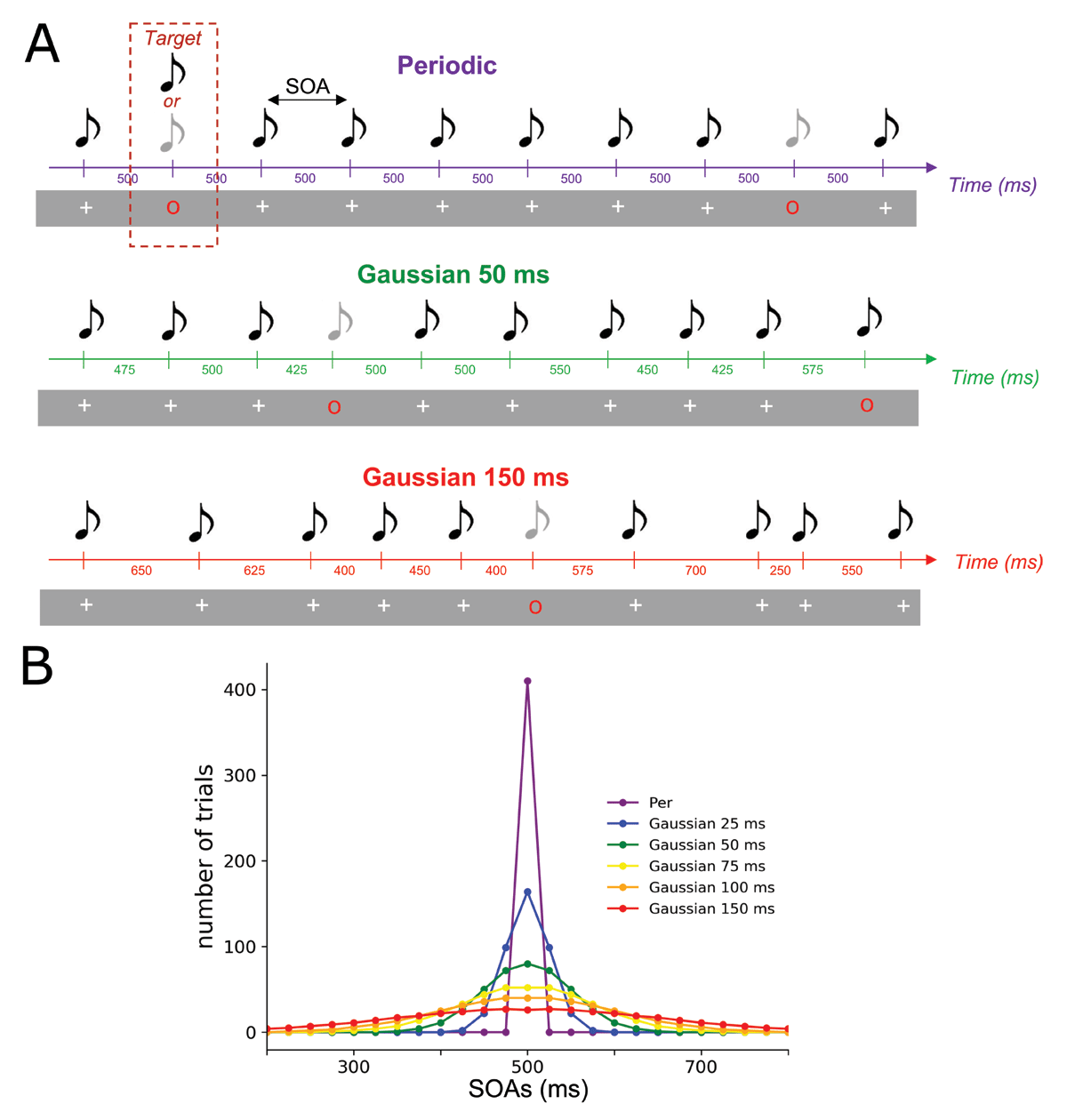
Figure 1
Experimental design. (A) Example of three sequences of different temporal STD used in this experiment. Each sequence consisted of a stream of simultaneous auditory and visual stimuli. A standard stimulus corresponded to a 440 Hz pure tone co-occurring with a white cross. Occasionally a red circle appears in the stream indicating a target stimulus, on which participants had to discriminate between a standard (440 Hz) and deviant (220 Hz) pure tone. (B) Distribution of SOAs in each sequence. For each sequence, the distributions of the SOAs were drawn of Gaussian distributions with equals means (500 ms) but distinct STDs. Six conditions were designed: from 0 (periodic) to 150 ms of STD with data points built from 100 ms to 900 ms and spaced from 25 ms.
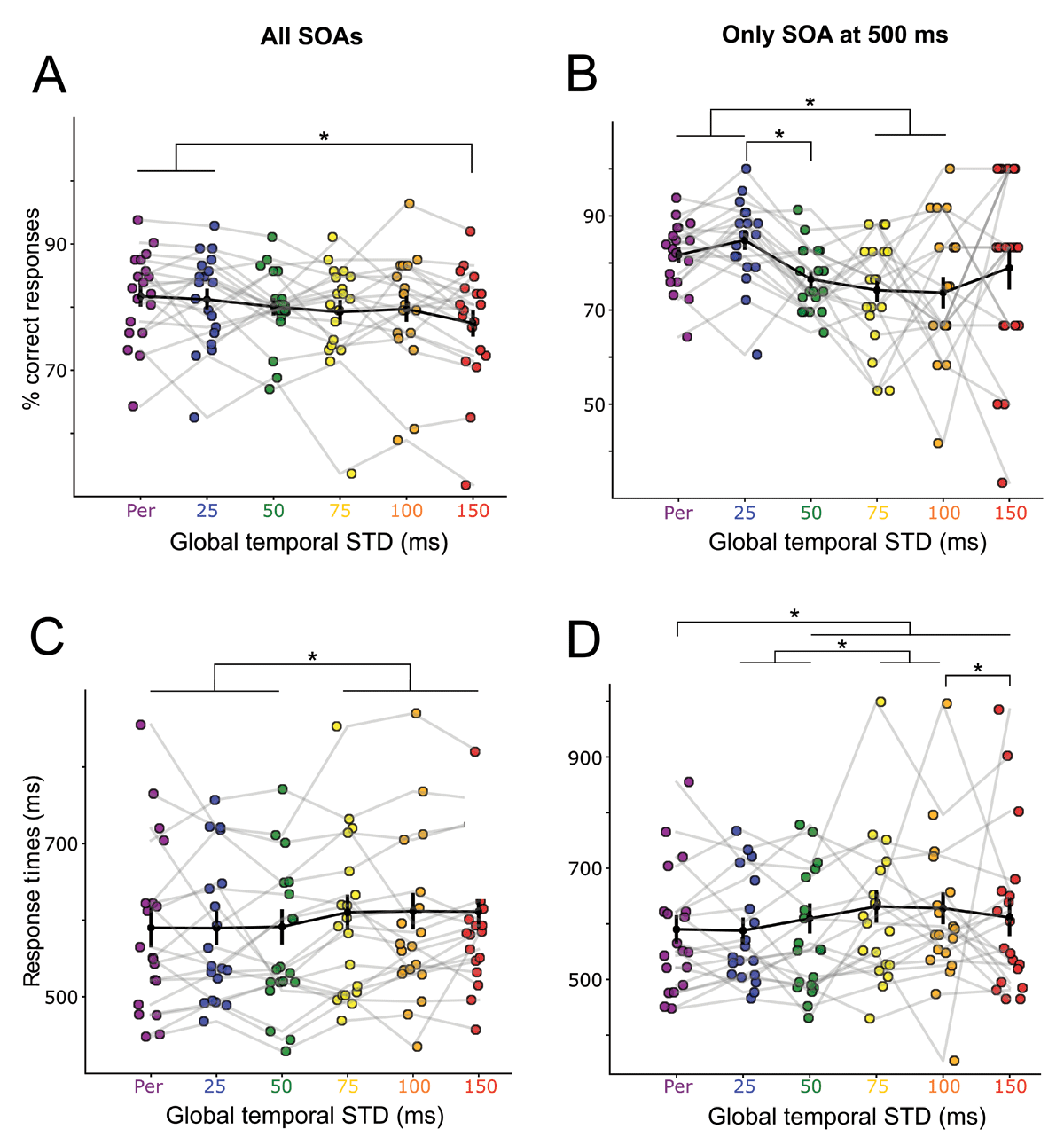
Figure 2
Auditory deviant discrimination is influenced by the temporal variability of the sound sequences. (A) Percentage of correct responses and (C) Response times as function of the standard deviation of SOAs in the auditory sequences. Each color dot represents a participant. Black dots represent the average across participants. Error bars indicate the Standard Error of the Mean (SEM) and stars indicate significant differences (p < 0.05). (B) Percentage of correct responses and (D) Response times restricted to target trials presented at SOA = 500 ms (mean of the distributions).
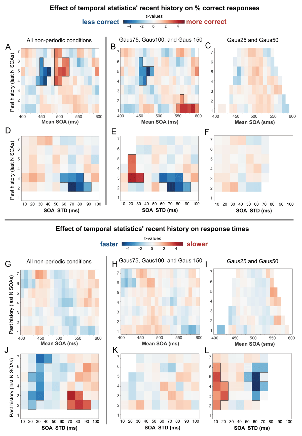
Figure 3
Effect of local temporal SOAs’ statistics on perception. The figures illustrate whether the relative performance of participants was affected by the mean and STD of the previous N SOAs. Specifically, we computed the mean and STD of the local SOA distribution drawn from the N previous SOAs before each target trial (with N ranging from 1 to 7 SOAs before target trial for mean SOA, and from 2 to 7 SOAs before target trial for SOA STD). We then binned target trials per SOA distribution mean (from 400 to 600 ms SOA mean, with a sliding window of ±20 ms length) and per SOA distribution STD (from 10 ms to 100 SOA STD, with a sliding window of ±10 ms length). Bins containing less than 5 trials per participant were excluded from further analysis. For each bin, the average accuracy and response time across trials was computed, and then z-scored across participants. The obtained 2-D plots represent whether accuracy and response times were relatively higher or lower depending on the mean and STD of the 2/3/4/… last SOAs. Data were aggregated for either (A, D, G, J) all non-periodic contexts, (B, E, H, K) the more variable temporal sequences (Gaus75 and higher), and (C, F, I, L) the less variable temporal sequences (Gaus25 and Gaus50 conditions). The color label represents the one sample t-test value against zero for each sample. Black lines denote significant clusters (transparency is applied to non-significant areas). Due to the low variability in conditions Gaus25 and Gaus50 some bins are left white (empty) because the number of trials was not sufficient to be representative (<5).
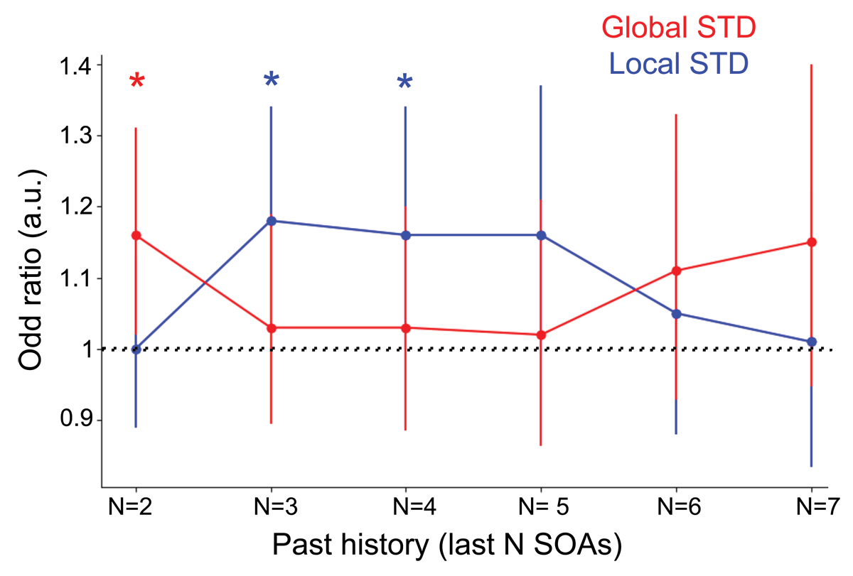
Figure 4
Interplay between local and global temporal SOAs’ STD on perception. We ran GLMMs that included both global STD and the local STD (from the N previous SOAs, N rating between 2 to 7) as predictors of subject’s response. The red line denotes the odds ratios of the global STD effect, the blue line denotes the odds ratio of the local STD effect, when local effects are computed with the N previous SOAs, N ranging from 2 to 7. An odds ratio superior to 1 means that participants were more correct for low STD trials than for high STD trials. Bars denote 95% confidence intervals, if the confidence interval is above 1 then the observed STD effects had a significant influence on the subject’s response. The models revealed an interplay between local and global STD effects. The local STD of the N previous SOAs did not have a significant influence on correct responses when N = 2 or N > = 5, while the global STD significantly biased perception. However, for N previous SOAs between 3 and 4 items, we observed that the local STD significantly influenced the subject’s response, while the influence of the global context relatively diminished.
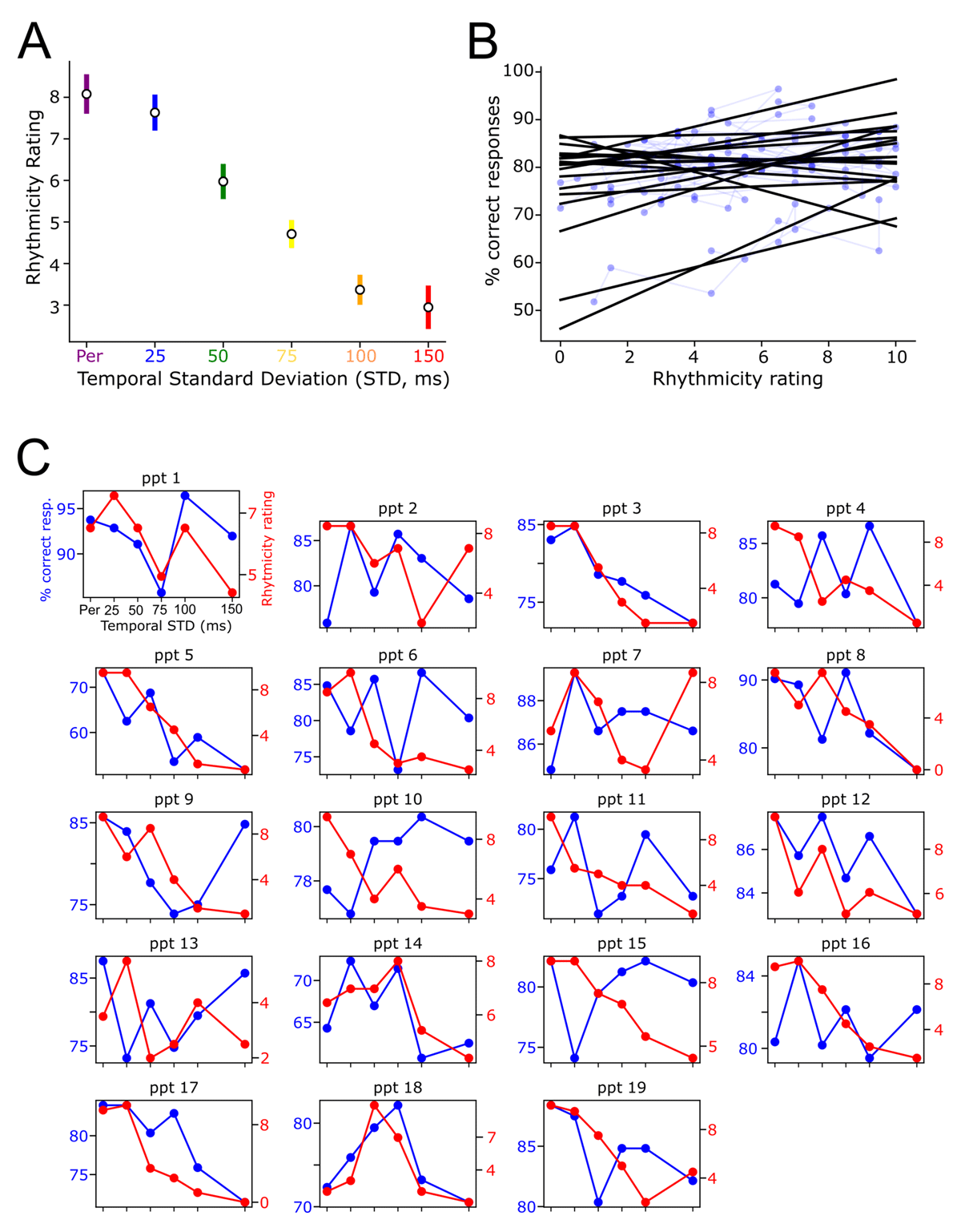
Figure 5
Link between subjective perception of rhythmicity and auditory performances. (A) Means of participant’s ratings of the degree of rhythmicity present in the temporal contexts. (B) Positive correlation between the rating and the percentage of correct responses. Each point and the corresponding regression line represent a single participant. (C) Individual correlations between percentage of correct responses and rhythmicity ratings. Each figure represents a participant’s data. Blue lines denote the percentage of correct response as a function of temporal standard deviation of sound sequences. Red lines denote the subjective rating of rhythmicity of each sound sequence.