
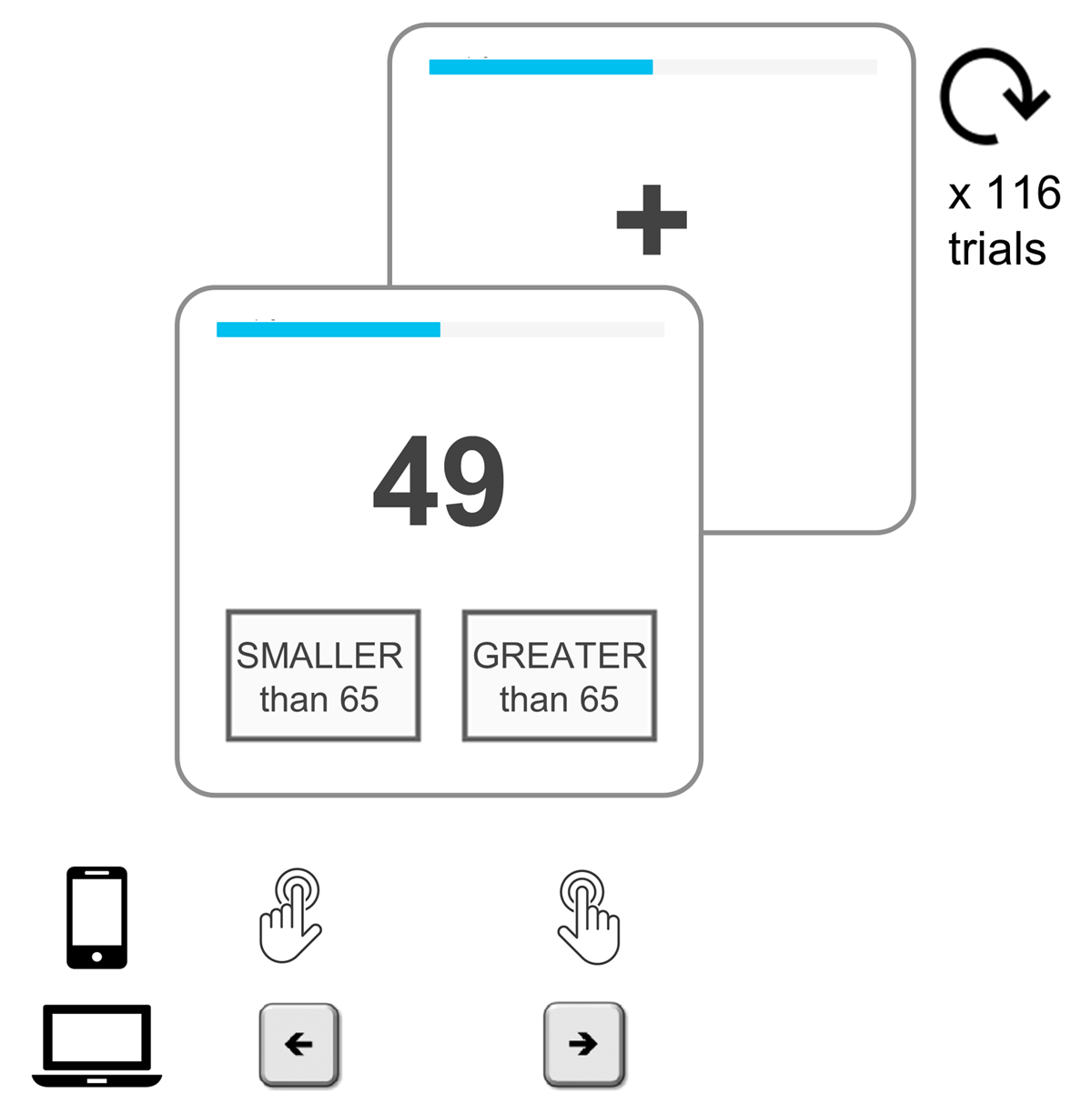
Figure 1
Number-comparison task. Participants had to decide whether a target number (49, in this case) was smaller or greater than a standard (65). We presented 58 target numbers: 29 were lower than the standard (from 36 to 64), and 29 were greater than the standard (from 66 to 94). Each of these targets was displayed twice, rendering a total of 116 trials. Trials were interleaved by an intertrial interval (ITI) that was randomly drawn from a uniform distribution (ITI ~ U(700 ms, 1000 ms)). Mobile device users responded on the screen by tapping a right or left box below the target, while desktop users responded by using the keyboard arrows. A left box tap/arrow keypress indicated a “smaller than 65” response and a right box tap/arrow keypress indicated a “greater than 65” response. On each trial, we recorded participants’ responses (smaller or greater) and response time (RT). Participants were instructed to be as accurate and fast as possible. To further enforce these instructions we applied a time deadline (each target was displayed for a maximum of 2 seconds) and a scoring system (+2 points for correct answers, –1 point for errors and timeouts). Finally, we included a progress bar (in light-blue at the top) to minimize dropouts due to uncertainty about how long the task would take.
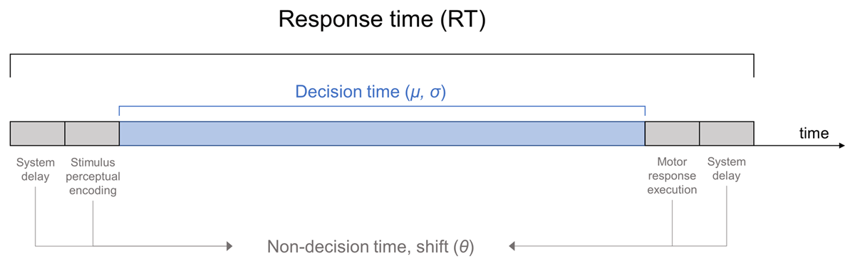
Figure 2
Temporal decomposition of the recorded response time (RT). On each trial, the recorded RT is the sum of a decision time and a non-decision time or shift (θ). The shift is assumed to represent both internal processes (perceptual encoding of the stimulus and motor response execution) and external delays. The latter are exclusively technological and include delays due to hardware, OS and browser processing speed, such as the latency between button, keypad or touchscreen press to the actual recording of the response. The decision time is the time the participant takes to evaluate the evidence, and it is assumed to follow a log-Normal distribution with parameters μ and σ.
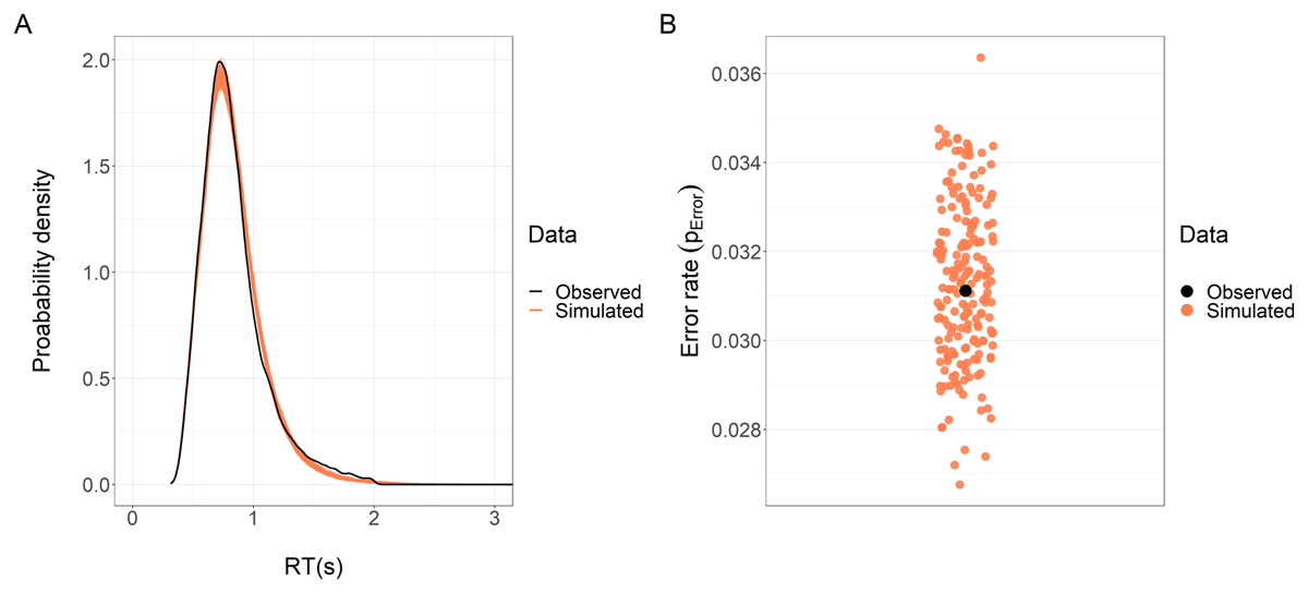
Figure 3
Posterior predictive checks for the RT and error rate models. (A) We simulated 200 datasets with the same structure as the observed dataset, using the RT model posterior distribution. We plotted the distribution of RT for each of these 200 simulations (light-red lines) and the observed RT distribution (black line). The high degree of overlap between the simulated and observed data distributions is indicative of the model’s ability to capture the distributional features of the observed RTs. (B) We performed a similar analysis for the error rate model but, since this variable is not continuous, we computed the mean error rate for each of the 200 simulated datasets (light-red dots) and for the observed data (black dot). Mean error rates from the simulated datasets are scattered around the observed error rate mean, which is indicative of the model’s ability to capture the main distributional feature of the observed error rate.
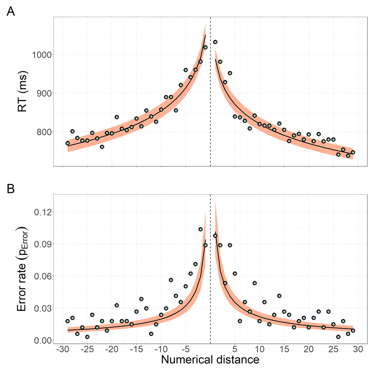
Figure 4
Numerical distance effect on RT and error rate. (A) Expected and observed values for RT as a function of the numerical distance between the target and the standard (distance is 0 at the dashed vertical line). Green dots are the observed overall mean of RT for each distance. The black line and shaded area represent the median and CI95 of the RT expected values (for an average participant), respectively, obtained from 2,000 model posterior samples. (B) Expected and observed values of error rate (i.e., probability of making an error) as a function of the numerical distance. Green dots are the overall proportion of errors for each distance. The black line and shaded area represent the median and CI95 of the expected values (for an average participant), respectively, obtained from 2,000 model posterior samples. Note that, as not all systems were equally represented in our data (e.g., there was only one session from an iPad device), we obtained and represented the weighted (by the frequency of the participants’ systems) marginal means for each distance in both panels. All means were computed for mean participants’ age and at mean trial number (i.e., at the middle of the task).
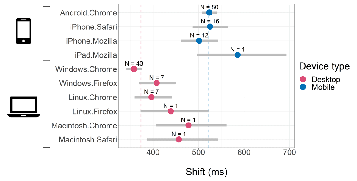
Figure 5
Shifts by participants’ system. We computed the conditional shift (θ) means by system (i.e., for each of the 10 categories of systems, see Methods) using 2,000 posterior samples from the estimated coefficients of the linear predictor of θ (Equation (3)). The colored points’ position and grey horizontal intervals represent the median and CI95 of the posterior samples for each conditional mean, respectively. We used dark pink and blue points to represent mobile and desktop devices, respectively, to show that mobile devices induce larger shifts than desktop devices. The annotation above each point reports the number of participants (N) that completed the task using that specific system. The dark pink and blue vertical dashed lines in the background are the shift means for mobile and desktop devices (weighted by the frequency of the participants’ systems, for each device type), respectively. All means were computed for mean participants’ age.
Table 1
Estimated Effects of the Participants’ System Over ν and σ.
| Distributional parameter | Coefficient | Median | Lower | Upper |
|---|---|---|---|---|
| ν | βsystem, Windows.Chrome | –0.009 | –0.037 | 0.019 |
| ν | βsystem, Windows.Firefox | –0.030 | –0.086 | 0.025 |
| ν | βsystem, Linux.Chrome | –0.041 | –0.097 | 0.015 |
| ν | βsystem, Linux.Firefox | 0.006 | –0.130 | 0.141 |
| ν | βsystem, Macintosh.Chrome | 0.010 | –0.126 | 0.148 |
| ν | βsystem, Macintosh.Safari | 0.025 | –0.125 | 0.178 |
| ν | βsystem, iPhone.Safari | –0.001 | –0.043 | 0.042 |
| ν | βsystem, iPhone.Mozilla | –0.012 | –0.057 | 0.033 |
| ν | βsystem, iPad.Mozilla | –0.061 | –0.210 | 0.095 |
| σ | γsystem, Windows.Chrome | –0.010 | –0.059 | 0.039 |
| σ | γsystem, Windows.Firefox | 0.037 | –0.052 | 0.123 |
| σ | γsystem, Linux.Chrome | –0.054 | –0.140 | 0.031 |
| σ | γsystem, Linux.Firefox | –0.090 | –0.229 | 0.047 |
| σ | γsystem, Macintosh.Chrome | –0.049 | –0.202 | 0.100 |
| σ | γsystem, Macintosh.Safari | 0.092 | –0.051 | 0.234 |
| σ | γsystem, iPhone.Safari | 0.044 | –0.027 | 0.111 |
| σ | γsystem, iPhone.Mozilla | –0.007 | –0.088 | 0.069 |
| σ | γsystem, iPad.Mozilla | 0.119 | –0.059 | 0.283 |
[i] Note: Lower and Upper refer to the lower and upper bounds of the CI95 of each coefficient posterior distribution. Importantly, all these intervals contain 0, suggesting that the participants’ system did not have a relevant effect on either μ or σ of RTs.