
Table 1
Moderator Analysis of Delay Between Sessions (reproduced from Dechêne et al. (2010) meta-analysis).
| SESSION 2 | K | D | 95% CI | Qb | ||
|---|---|---|---|---|---|---|
| LOWER BOUND | UPPER BOUND | |||||
| Within-items | 3.44 (2.74) | |||||
| Within day | 9 | .25 (.24) | 0.07 (0.04) | 0.43 (0.46) | ||
| Within week | 11 | .44 (.45) | 0.31 (0.29) | 0.57 (0.61) | ||
| Longer delay | 10 | .44 (.45) | 0.32 (0.28) | 0.56 (0.61) | ||
| Between-items | <1 (<1) | |||||
| Within day | 25 | .48 (.49) | 0.39 (0.37) | 0.57 (0.62) | ||
| Within week | 14 | .43 (.44) | 0.32 (0.28) | 0.54 (0.59) | ||
| Longer delay | 12 | .48 (.49) | 0.36 (0.32) | 0.59 (0.65) | ||
[i] Note: Fixed-effects values are presented outside brackets, and random-effects values are within brackets. Within-items = the difference in ratings for repeated statements between exposure (session 1) and test phase (session 2). Between-items = the difference between truth ratings for new versus repeated statements during the test phase. For within-items, within day is descriptively smaller, however delay did not modify either within-items or between-items as shown by the non-significant goodness of fit statistic Qb.
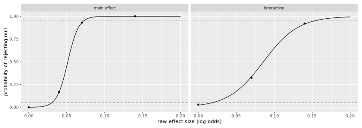
Figure 1
Estimated sensitivity curves for a sample with a final N of 440 participants (based on a starting N of 608 with dropouts). Each point in the plot was based on 100 simulations, and the curves were obtained by fitting a logistic regression model to the data. For reference, the dashed line is at the 5% null rejection rate and the dotted line is at the 95% rejection rate.
Table 2
Sequence of Application of Preregistered and Non-Preregistered Exclusion Criteria.
| APPLICATION ORDER | EXCLUSION CRITERIA |
|---|---|
| Participant-level | |
| 1 | Duplicate sessions recorded* |
| 2 | Consent to data collection across all four phases was absent* |
| 3 | English not first language |
| 4 | Used technical aids to answer question(s) |
| 5 | Responded uniformly across an entire phase of the study |
| 6 | Failed to complete all phases in a reasonable amount of time |
| 7 | No ratings data* |
| 8 | Other: participant asked for their data to be withdrawn* |
| Phase-level | |
| 9 | Consent for phase was absent* |
| 10 | Failed to complete all of the ratings in the phase |
[i] Note: Non-preregistered criteria are marked with an asterisk. “No ratings data” means that there was no more data left for that subject following application of the phase-level exclusion criteria. This occurred if, for example, a participant partially completed phase 1 before dropping out. Data for that phase would be excluded based on the phase-level criterion “Failed to complete all of the ratings in the phase”, leaving no ratings data for that participant at all, and so we also deleted their participant-level information.
Table 3
Participants Recruited, Excluded, Retained, and Analysed, Separated by Experimental Phase and Gender.
| PHASE | GENDER | N RECRUITED | N EXCLUDED | N RETAINED | N ANALYSED |
|---|---|---|---|---|---|
| 1 | Female | 386 | 6 | 380 | 364 |
| Male | 212 | 8 | 204 | 198 | |
| Gender variant | 2 | 0 | 2 | 2 | |
| Prefer not to say | 3 | 0 | 3 | 3 | |
| (Missing) | 28 | 28 | 0 | 0 | |
| TOTAL | 631 | 42 | 589 | 567 | |
| 2 | Female | 365 | 10 | 355 | 346 |
| Male | 201 | 2 | 199 | 194 | |
| Gender variant | 1 | 0 | 1 | 1 | |
| Prefer not to say | 3 | 0 | 3 | 3 | |
| (Missing) | 4 | 0 | 4 | 0 | |
| TOTAL | 574 | 12 | 562 | 544 | |
| 3 | Female | 347 | 7 | 340 | 337 |
| Male | 197 | 1 | 196 | 191 | |
| Gender variant | 1 | 0 | 1 | 1 | |
| Prefer not to say | 3 | 0 | 3 | 3 | |
| (Missing) | 3 | 0 | 3 | 0 | |
| TOTAL | 551 | 8 | 543 | 532 | |
| 4 | Female | 329 | 7 | 322 | 322 |
| Male | 192 | 9 | 183 | 183 | |
| Gender variant | 0 | 0 | 0 | 0 | |
| Prefer not to say | 2 | 0 | 2 | 2 | |
| (Missing) | 3 | 0 | 3 | 0 | |
| TOTAL | 526 | 16 | 510 | 507 |
[i] Note: “Missing” refers to participants who did not finish phase 1 and therefore did not report their gender. Four of these participants were erroneously invited back to future phases because they started multiple sessions at phase 1. Participants who started multiple sessions during any phase were excluded from analyses. “N retained” is the number of participants after exclusions were applied at the end of each phase. “N analysed” is the number of participants after exclusions were retroactively applied. For example, if a participant responded uniformly to all statements during phase 4, their data were excluded from all previous phases.
Table 4
Summary of Exclusions, Dropouts, and Attrition by Phase.
| PHASE | RECRUITED | ATTEMPTED | EXCLUDED | RETAINED | ANALYSED | DROPOUT | EXCLUDED | ATTRITION |
|---|---|---|---|---|---|---|---|---|
| 1 | NA | 631 | 42 | 589 | 567 | NA% | 10.1% | NA% |
| 2 | 589 | 574 | 12 | 562 | 544 | 2.5% | 5.2% | 7.7% |
| 3 | 566 | 551 | 8 | 543 | 532 | 2.7% | 3.4% | 6.1% |
| 4 | 545 | 526 | 16 | 510 | 507 | 3.5% | 3.6% | 7.1% |
[i] Note: “Retained” is the number of participants after exclusions were applied at the end of each phase. “Analysed” is the number of participants after exclusions were retroactively applied. For example, if a participant responded uniformly to all statements during phase 4, their data were excluded from all previous phases.
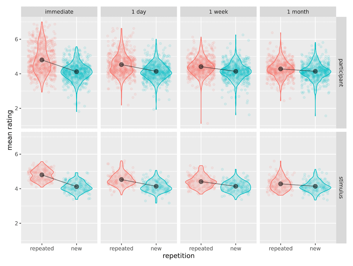
Figure 2
Effect of repetition across interval, cell means (black points, line) plotted against participant means (top row) and stimulus means (bottom row).
Table 5
Mean Ratings and SDs for Repeated Versus New Statements, and Their Difference, by Interval.
| INTERVAL | REPEATED M (SD) | NEW M (SD) | DIFFERENCE |
|---|---|---|---|
| immediately | 4.80 (1.54) | 4.12 (1.36) | 0.68 |
| 1 day | 4.53 (1.45) | 4.14 (1.36) | 0.39 |
| 1 week | 4.41 (1.38) | 4.14 (1.33) | 0.27 |
| 1 month | 4.28 (1.37) | 4.14 (1.32) | 0.14 |
Table 6
Planned Comparisons of the Simple Effect of Repetition at Each Interval, with Holm-Bonferroni Correction.
| CONTRAST | INTERVAL | ESTIMATE | SE | Z RATIO | REJECT NULL |
|---|---|---|---|---|---|
| repeated – new | Immediately | 1.04 | 0.05 | 22.68 | True |
| repeated – new | 1 day | 0.56 | 0.03 | 18.64 | True |
| repeated – new | 1 week | 0.37 | 0.03 | 11.00 | True |
| repeated – new | 1 month | 0.20 | 0.04 | 5.53 | True |
Table 7
Summary of Experimental Design from Research Questions to Results.
| QUESTION | HYPOTHESIS | TEST NO | ANALYSIS PLAN | POWER ANALYSIS | RESULTS |
|---|---|---|---|---|---|
| Is there a time-invariant illusory truth effect? | H1: We will observe a main effect of repetition averaging across all four delay durations. | 1 | Fit a cumulative link mixed model (as detailed in the “Simulated Data & Analyses” component on the OSF) and conduct χ2 test with one degree of freedom, with α = .05. | 95% power to detect an effect of .07 or larger on the log odds scale (about a twentieth of a scale point on a seven-point scale). Based on 440 participants completing phase 4. | Supporting H1, there was a significant main effect of repetition when collapsing over interval, (SE = 0.04), χ2(1) = 171.88, p < .001. |
| 2 | IF tests 1 and 3 are non-significant: Test for the absence of the main effect using an equivalence test with bounds of ΔL = –0.14 and ΔU of 0.14 on a log odds scale. | 95% power to reject the null of a raw effect greater than .085. | |||
| Does the illusory truth effect vary over time? | H2: We will observe a repetition-by-interval interaction such that the size of the illusory truth effect will differ across the delay durations. | 3 | Fit a cumulative link mixed model (as detailed in the “Simulated Data & Analyses” component on the OSF) and test the repetition-by-interval interaction using a χ2 test with three degrees of freedom and α = .05. | 95% power to detect an effect of a tenth of a scale point, (about.14 on the log odds scale) between two arbitrarily chosen time points: If an illusory truth effect only emerges at very the last time point, we can detect it with 95% power as long as it is at least a tenth of a scale point. Based on 440 participants completing phase 4. | Supporting H2, there was a significant repetition-by-interval interaction, (SE = 0.05; immediately vs. one day), (SE = 0.07; immediately vs. one week), (SE = 0.07; immediately vs. one month), χ2(3) = 121.15, p < .001. |
| 4 | IF test 3 is significant: Use emmeans() to attempt to localise the effect, testing the effect at each of the four intervals, and using a Holm-Bonferroni stepwise procedure to keep the familywise error rate at .05. | N/A | Pairwise comparisons revealed that at every interval, estimated marginal means for repeated statements were significantly higher than those for new statements, indicating that the illusory truth effect was present at all four phases (Table 6). | ||
| 5 | IF test 3 is non-significant: Test for the absence of an interaction effect using an equivalence test considering all six possible pairwise comparisons of the illusory truth effect across intervals to see whether they fall within the bounds of ΔL = –0.14 and ΔU of 0.14 on a log odds scale | With |Δ| =.14, 37% power to reject H0 if the true value is 0, about 18% power if true value is .07 or smaller. With |Δ| =.20, 93% power if the true value is 0, 75% power if the true value is .07 or smaller, 18% power if the true value is .14 or smaller. For results with .14 < |Δ| < .20, see equivtest.html in the repository. |
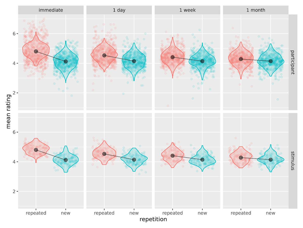
Figure 3
Model validation: Plot of observed participant/stimulus means (points) against simulated data distributions (violins) and cell means (black points, line).
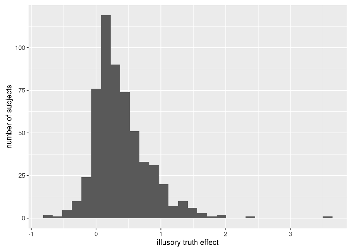
Figure 4
Distribution of participants showing an overall effect of the illusory truth effect.
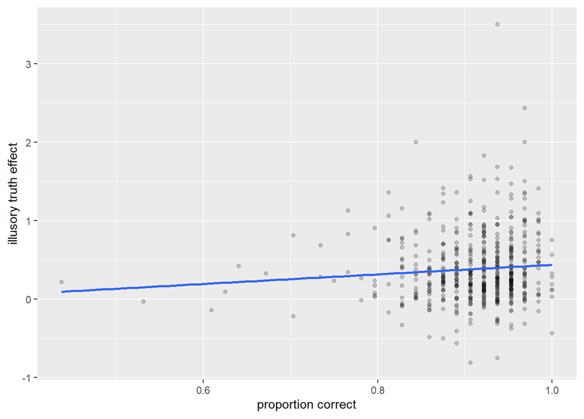
Figure 5
Illusory truth effect by category judgment accuracy.
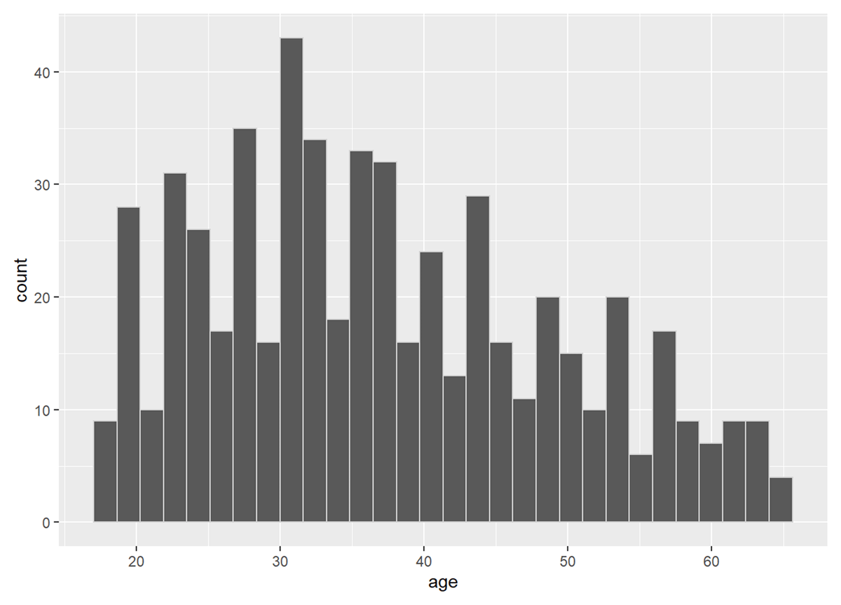
Figure 6
Distribution of participants’ age.
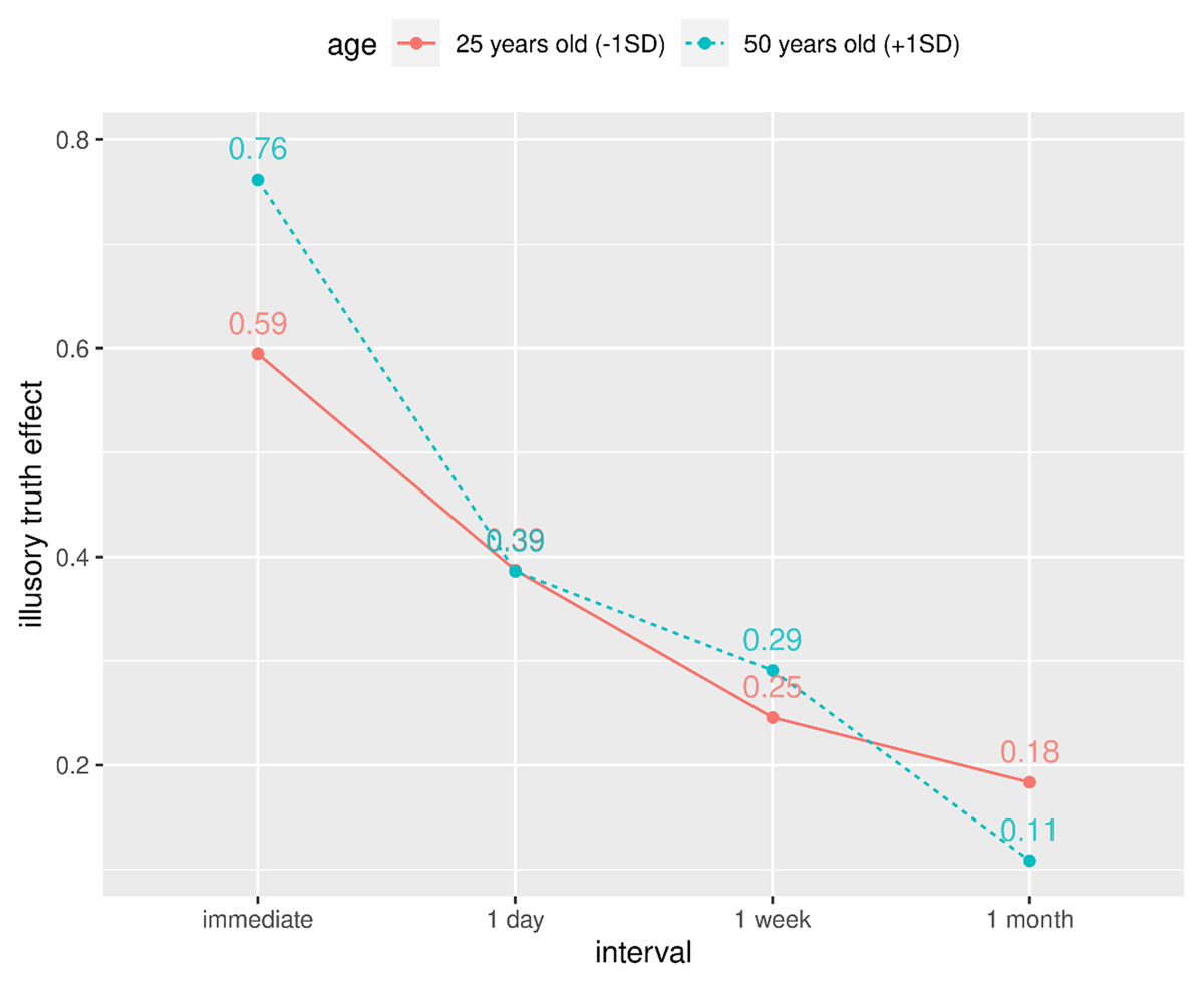
Figure 7
Model predictions for the trajectory of the illusory truth effect for two ages.