
Introduction
In the practice of archaeological fieldwork, new technologies are continuously introduced. Whereas this is a long and ever-present tradition, also for digital technology (e.g., Pollefeys et al. 2001; Neubauer & Doneus 2005), its pace has significantly quickened. Especially in the last two decades or so, this has led to a substantial increase in the development of digital workflows at archaeological excavations, with a large emphasis on 3D recording (Olson et al. 2013; De Reu et al. 2014; Roosevelt et al. 2015; Dell’Unto et al. 2017; Nobles & Roosevelt 2021; Badillo et al. 2024). In general, these workflows are often referred to as ‘paperless archaeology’ (e.g., Wallrodt 2016), where digital recording methods replace the traditional paper-based techniques using analogue forms, lists, drawings, etc. Such approaches encompass, e.g., the use of tablets for record entry and digital drawing, (drone-) photogrammetry for 3D recording of archaeological contexts, multiuser database setups, and/or automatic Harris-matrix generation (Boyd et al. 2021), and can be expected to converge with prospection/sensor approaches to the excavation trench (e.g., geophysical prospection: Leucci, De Giorgi & Scardozzi 2014; drone remote sensing: Waagen & van Hilst 2025; or XRF applications: Williams, Errickson & Taylor 2021).
The introduction of these digital workflows is expected to increase efficiency through direct digitization, improve data quality because of accurate recording technology and more formalized procedures, introduce democratization of access to excavation data, and allow for faster interpretation cycles allowing for more on-site reflection, to name a few important ones. Their introduction also raised critical questions though, regarding both potentially positive as well as negative effects on the recording and associated knowledge production process. Several main discussion topics can be discerned, relating to either practical, technical, procedural, and theoretical considerations. One example pertains to the incorporation of digital workflows within established excavation methodologies and processes. This raises the question to which extent the introduction of these novel techniques may disrupt the continuity of excavation operations and whether such integration necessitates a level of expertise that is both substantial and potentially particularly expensive (cf. Waagen 2019; Boyd et al. 2021). Another, more theoretical topic relates to how the affordances of the specific tools affect the process of knowledge production. How do they support archaeological fieldwork as a reflexive practice (Berggren et al. 2015), where the deployment of digital tools is also potentially limiting (Caraher 2016; Morgan & Wright 2018), including to its pedagogical potential (Morgan et al. 2021)? As such, it is imperative to emphasize that, in the end, digital tools must facilitate the construction of archaeological knowledge (Berggren & Gutehall 2018). In a more practical and technical sense: how do we ensure quality, both in terms of collecting accurate data that is fit for purpose, as well as in adhering to standards in terms of software, formats, and data standards, such as the FAIR principles (Ross et al. 2022; Wilkinson et al. 2016), and fully work towards transparent and Open Access workflows that are platform independent? In all these directions, the discourse in the field of archaeology is advancing.
While acknowledging the comprehensive methodological and theoretical developments in fieldwork practices, a key element in progressing toward ‘reflective paperless archaeology’ is the adoption of data capture methodologies that are efficient, cost-effective, and accessible. In the context of fieldwork of the Amsterdam Center for Ancient Studies and Archaeology of the University of Amsterdam, as in many other archaeological institutes, there has been continuous development and experimentation with innovative digital fieldwork technology. At the archaeological site of ancient Halos (Thessaly, Greece), a solid workflow for capturing the archaeological excavation effort in detail has been implemented. This site has been investigated in the Halos Archaeological Project of the Amsterdam Center for Ancient Studies and Archaeology, in collaboration with the Ephorate of Magnesia, the University of Groningen (until 2023) and the University of Thessaly (Reinders 1988; Stissi et al. 2015; 2020). In an earlier paper, a drone photogrammetry approach was discussed, designed to be non-disruptive to the ongoing archaeological process, as well as adhering to required data standards, and well-integrated into the documentation procedures and standards of the project (Waagen 2019). At the site of Halos, the workflow procedure was further developed using a multi-user database accessible through tablets in the field, that also allow for full QGIS data access and sketching tools. The drone recording takes place after fieldwork late in the afternoon, to profit from equal lighting conditions (i.e., avoiding cast shadows) as well as not interfering with the excavation process. The downside to this workflow however is that all intermediate excavation actions are not documented. Ideally, every documentation moment part of the excavation workflow that requires drawing and digital photographing should also be incorporated in the 3D scanning. Otherwise, it is theoretically possible that, e.g., smaller stratigraphical units that can be excavated and documented in the course of two to three hours will not be captured in the daily drone photogrammetry documentation. Therefore, it is vital for this workflow to develop a solution for intermediate 3D recording of archaeological contexts, again focusing on limiting the impact on the ongoing archaeological excavation process.
The above-mentioned literature of course also deals with various approaches from incorporating terrestrial LiDAR and structure from motion approaches (Neubauer & Doneus 2005; Olson et al. 2013). However, a terrestrial LiDAR scanner is associated with high costs, disruption of the excavation process, and most of all, it is difficult to specifically target at smaller contexts and avoid obfuscation of parts of the trench depending on the topography of the excavated remains. Photogrammetry is inherently versatile due to its adaptability. However, it necessitates a significant level of data capture expertise and can at times be cumbersome in the field. Additionally, the data processing involved can be time intensive. Increasingly, other options for relatively mobile approaches to 3D surface recording are available, for example with wireless handheld structured light scanners such as the Artec Leo (Artec Leo 2025). The relatively recent appearance of the iPhone LiDAR sensor potentially lowers the threshold even further (Brookes 2022), as it is a relatively easy and affordable technology with a potentially high-quality output. As these technologies are used on many projects it is important to develop a good understanding of their absolute and relative qualities.
Research aim
The remainder of this paper focuses on comparing three different 3D capture techniques: photogrammetry, structured light scanning, and low-cost LiDAR. The study provides a comparative analysis of these technologies, focusing on several critical dimensions. Specifically, it will evaluate the requisite level of expertise for effective utilization, the practical applications with particular attention to ergonomic considerations, the processing time involved, and the precision and accuracy of the data produced. This evaluation will encompass both geometric quality and the fidelity of texture (color) representation.
Review of previous work
The techniques discussed in this paper have been evaluated and compared in previous studies. The iPhone LiDAR has been tested as cost-effective alternative for professional scanning equipment in the context of fieldwork on a tight budget in geology (Luetzenburg, Kroon & Bjørk 2021; Furlan & Piazentim 2025), building history (Abbas & Abed 2024) and archaeology (Paukkonen 2023). The results of these tests are generally positive, with the iPhone LiDAR being a cheap, time-efficient and user-friendly method for 3D data capture where cm accuracy is sufficient. Luetzenburg and fellow researchers tested the first-generation iPhone 12 LiDAR on a rock cliff 130 m long and 10 m high. They found that 80% of points are within 15 cm and 96% within 30 cm of the Structure from Motion (SfM)-based reference point cloud. On smaller 10 by 10 m sections of this cliff scanned at closer range, this deviation was reduced to 5 cm at 92% of the points. The iPhone 12 LiDAR unit was also tested by Abbas & Abed (2024) using an experimental setup of a purpose-built wall with 8 by 8 cm targets pinned on in a grid. This wall was scanned by both a terrestrial laser scanner (Stonex X300) and the iPhone at 4.60 m distance. The targets, serving as ground control points, were measured using a Total Station. The remote square error resulting from both scanners was very close (RMSE TLS: 3.44 mm vs RMSE iPhone: 4.89 mm). The distance effect observed by Luetzenburg et al. (2021) was also confirmed by these authors, revealing a linear pattern with a RMSE at close range (0.25 m) of 2 mm, to 5 mm at maximum range (5 m). The authors conclude that the iPhone LiDAR is capable of mm accuracy.
Furlan & Piazentim (2025) tested the iPhone 15 with an improved LiDAR unit. They confirmed the observation by previous authors that distance to target had a significant effect on the accuracy of the scan. They focused, however, on the capability to make manual measurements of small features on rock outcrops, using tape-measured data as reference. Due to the sparsity of the iPhone-produced cloud, these features could not be measured effectively at all ranges. At 0.3 m it is the most accurate, but less time-efficient in capturing medium-sized geological features. Only at this range, features smaller than 1 cm could be effectively measured. At 2.5 m distance a good balance is struck between time-efficiency and accuracy. At its maximum scanning range (5 m) it is the most inaccurate and does not reduce capturing times as much as between the 0.3 m to 2.5 m ranges. They moreover compared eight different scanning apps for the iPhone, concluding that only two (Scaniverse and PolyCam) gave acceptable results, with Scaniverse being the superior app. It is noteworthy that the app used by Abbas & Abad (2024), SiteScape, resulting in mm accuracy, was not deemed usable by Furlan & Piazentim (2025). This suggests that test outcomes may be strongly determined by the chosen capturing setup and/or type of captured object.
Paukkonen (2023) delivered a test of the iPhone on an archaeological case. This study compares the iPhone LiDAR (using both the Scaniverse and Pix4D Catch apps) with photogrammetry using a Dji Osmo Pocket, and a Riegl VZ-400i TLS. Clouds were aligned without ground control points, and statistical differences computed using the M3C2 algorithm in CloudCompare. The results were assessed against 2 cm and 5 cm accuracy thresholds considered acceptable for archaeological documentation. Photogrammetry with the DJI Osmo Pocket had 90.2% of measured points fall within the 5 cm accuracy range, 58.4% for the iPhone with the Pix4D app and 59.1% for the Scaniverse app. Volumetric measurements also showed significant inaccuracies. The author concludes that the iPhone LiDAR is not recommended for precise archaeological documentation but is useful for quick data capture for non-scientific visualization. Where others judged the iPhone LiDAR usable and accurate, Paukkonen assesses it to be too inaccurate for scientific archaeological analysis and only suitable for illustration purposes.
The results of these studies are diverging, as is their assessment of the usability of the iPhone LiDAR in the respective fields of study. The different data capture setups and methods of assessing the data make it hard to compare the results and may be the cause for inconsistent results. It is therefore useful to continue testing this sensor, in order to understand its capabilities in specific contexts and conditions.
Technologies for flexible mobile 3D data capture
For the first technique, structure from motion, commonly referred to as photogrammetry, a midlevel DSLR photo camera with prime lens was chosen. This represents a capturing device typically available on archaeological fieldwork projects, and for many teams constitutes a logical and affordable solution for mobile 3D data capture. Common uses of photogrammetric documentation are the generation of a sequence of textured 3D models of an excavation trench, and georeferenced orthophotos. The latter play an important role in the fieldwork project’s GIS system, used amongst others as reference for the drafting of excavation plans. However, photogrammetry takes time and skilled operators in the field, as the images need to be captured respecting a few technical principles (fixed aperture, focus and depth of field optimisation, equal distance to object, redundant overlap between photos; see, e.g., Sapirstein & Murray 2017).
As an alternative to photogrammetry, since 2022, experiments have been conducted by the 4D Research Lab with the aforementioned Artec Leo scanner, a mobile structured light 3D scanning device. Structured light scanners project a calibrated pattern of light on a surface, which is captured by one or two depth sensors (cameras) and reconstructed in the software by means of triangulation. The Artec Leo (Lievendag 2017; Madeleine 2021) uses a less conventional laser light emitter (VCSEL) to project an invisible pattern. This means that this scanner performs better in bright conditions than scanners that work with a visible light source. It has an NVIDIA® JetsonTM TX1 processor which enables real-time feedback and interactive previewing of the data. It is a completely mobile platform, able to position itself in space thanks to its accelerometer, gyroscope and compass. This is a less affordable solution, but offers high-speed scanning, calibrated accuracy, and state-of-the-art processing software. Finally, a low-cost solution has seen increased application in recent years, which is the Apple iPhone or iPad with integrated LiDAR sensor (Paukkonen 2023). Like the Artec Leo, this offers fast scanning and reasonable accuracy (see review of previous work above) in addition to easy-to-use processing software. The latter reduces the number of options and control over the final product but substantially lowers the costs as well as the threshold for non-technical users (for details on all three devices, see Table 1). Users will have to choose between multiple available apps for the iPhone LiDAR. Based on recommendations of colleagues we opted for PolyCam. Although in the comparison of eight apps made by Furlan & Piazentim (2025) PolyCam ended second best after Scaniverse, this data was not available to us at the time of our experiments.
Table 1
Technical details of data capture devices. Technical details on the iPhone LiDAR sensor are not shared by Apple. The listed details are derived from tests by Luetzenburg, Kroon and Bjørk (2021). Since they tested an earlier version of the device, the iPhone 12 versus our iPhone 15, these details may differ.
| DEVICE | TECHNIQUE | SENSOR | ACCURACY | RESOLUTION/PRECISION | EFFECTIVE CAPTURE RANGE | PRICE DEVICE € (2025) | PRICE SOFTWARE |
|---|---|---|---|---|---|---|---|
| iPhone(Sony IMX 591 LiDAR SPAD) | LiDAR with sensor fusion (multiple device sensors) | VCSEL (emitter), SPAD (receiver) Fusion with other device sensors (camera lenses, accelerometer, gyroscope, and magnetometer | 1–10 cm depending on distance to subject | 0.01 megapixel | 0.3–5.0 m | Ca. 1.5k | Free 12,50 p/m (basic license) |
| Nikon D5300 | Photogrammetry | Size: APS-C (23.5 × 15.6 mm) Type: CMOS | Relies on external measurement | 24 megapixels/depends on distance | 0.4–100 m | Ca. 1k | 529 (educational) 3370 (regular) |
| Artec Leo | Structured light | VCSEL (pattern emitter), depth and texture camera specs not provided | 0.1 mm point | 0.2 mm point | 0.35–1.2 m | Ca. 30k (educational) | 2 years included (educational pack) 100 p/m (regular subscription) |
Data capture and processing
Data capture
At the excavation trench, a section of a profile adjoining a floor surface was selected for study. Measuring approximately 2.0 m by 0.5 m, this area includes an excavated surface and a vertical portion of an irregular profile with stones and ceramic material that was considered representative of the typical geometric complexity found in habitation context excavations in this region. The data for the three compared techniques was captured in close temporal sequence, to guarantee similar conditions (Figure 1). Early morning was chosen as an ideal time, as the diffuse lighting and absence of high contrasts resulting from sunlight and cast shadows results in evenly lit textures on the 3D models. The data capture took ca. 20 minutes in total by experts with experience using all three techniques. The settings were optimized for outdoor capture based on earlier experimentation (capture details in Table 2).
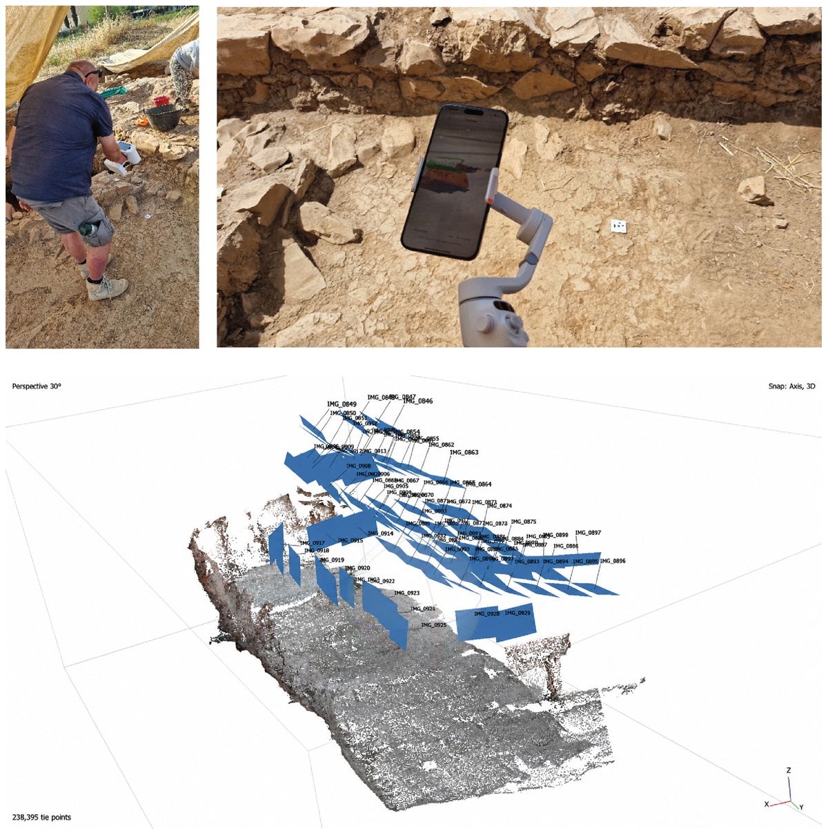
Figure 1
3D data acquisition in the field. Upper left: the Artec Leo. Upper right: the iPhone (photos Jitte Waagen). Lower: positions of the photos captured for photogrammetry.
Table 2
Data capture details.
| DEVICE | CAPTURE SETTINGS | CAPTURE TIMES | DATA SIZE |
|---|---|---|---|
| iPhone 15 pro Max with DJI Osmo Mobile 6 | PolyCam scan settings: lidar object scanning Shutter: Auto Mode | 2 min | Exported .laz file: 21 mb Exported 3D model: 38 mb |
| Nikon D5300 Nikon 35 mm prime objective | Data type: JPG Resolution: 0.8 mm/pix (reprojection error 0.75 pix) White balance: auto Aperture: f/4.5 ISO: auto Shutter time: auto FL: 35 mm | 15 min | Number of photos: 84 Exported 3D model: 10 GB |
| Artec Leo | HD data: no Data framerate: 60 fps Supplementary texture: 8 fps | 2 min | Size of raw data: 9.33 GB Exported 3D model: 1 GB |
| Differential GPS (dGPS): GCX3 Sokkia Bullet GNSS base/rover | N/A | 1 min | N/A |
For the purpose of geolocating and, in the case of photogrammetry, scaling the scans, dGPS measurements were taken on targets that were used as Ground Control Points (GCPs). In addition, 20 supplementary points were measured to serve as control points (CTRs). The GCPs will be included in the data processing workflows for scaling and geolocation, while the CTRs will be kept aside and later used for error assessment in comparing the relative accuracy of the models.
Data processing
The hardware/software setup for all the processing was done on a relatively high-end gaming laptop (Table 3).
Table 3
Technical details of processing laptop.
| LAPTOP | SPECIFICS |
|---|---|
| Processor | Intel Core i9-12900HX, 16 cores |
| Graphics Card | GeForce RTX 3080 Ti, 16 GB |
| Processing memory | 32 GB RAM DDR5 |
| Operating System | Windows 11 Pro |
All photogrammetry data collected with the Nikon D5300, stored locally on the removable SD card, was processed using Agisoft Metashape (Agisoft Metashape 2025), software chosen on the basis of on long-time familiarity. We applied a proven workflow, consisting of subsequently importing all photos as cameras, aligning them to produce a sparse point cloud, densifying the point cloud, building a mesh, a texture, and finally an orthomosaic (details in Table 4). Scaling and geolocating can be done directly in the software by incorporating the target coordinates measured with the dGPS.
Table 4
Technical details of Agisoft Metashape processing.
| ALIGN | POINT CLOUD | MODEL | TEXTURE | ORTHOMOSAIC |
|---|---|---|---|---|
| Generic preselection, High accuracy, Key point 40k, Tie point 4k | Depth Maps source, High quality, Mild Depth Filtering | Point Cloud source, Arbitrary Surface Type, 200.000 face count, Interpolation enabled | Diffuse Map, Image source data, Default Blending Mode, texture size 8192, enabling Hole Filling and Ghost Filter | Model Surface, Default Blending Mode, enable Hole Filling, Default Pixel Size |
All data collected with the iPhone, LiDAR point cloud and photos, is stored locally on the device. The LiDAR data can immediately be processed, also taking place directly on the iPhone in PolyCam, which warms up considerably during the process. It took around 2 minutes to process a mesh with maximized detail, consisting of a mesh of 287.692 polygons with 4K textures. The actual processing parameters remain hidden to the user, rendering this a so-called ‘black box’ technology (Bunge 1963). The output mesh was geolocated in CloudCompare, using a workflow described below.
Finally, the structured light data collected with the Artec Leo is also stored locally and can be exported after fieldwork using a USB-C cable. To process this data proprietary software Artec Studio is required. In the Artec Studio 17 (Artec Studio 2025) software, the scan is first registered, then manually checked for erroneous/superfluous frames, worked into a mesh using fusion, and textured (Table 5). The raw scan data is preserved after the project, although it must be noted that this is a proprietary data format not readable without the Artec Studio software. The fused and textured mesh is exported from the software to widely used 3D data formats and used for further processing and analysis.
Table 5
Technical details of Artec Studio processing.
| REGISTRATION | ALIGN | FUSION, TEXTURE |
|---|---|---|
| Global registration: collective, Key frame ratio 0.1, Search features within, mm 15, Smart subsampling turned on | If applicable (multiple scans): manual first, then automatic | Smart fusion (sharp) on each scan, and apply texture |
As neither Leo nor iPhone offers options to assign world coordinates to their outputs, this data was georeferenced after export in open-source software CloudCompare (CloudCompare 2025). Georeferencing in CloudCompare is enabled by the mesh to cloud align tool. The mesh of the scan is loaded as ‘to be referenced’, while the measured dGPS targets were loaded in the software as reference ‘cloud’. The meshes were manually referenced by matching the dGPS points with the GCPs in the scans. This was based on the visibility of the targets on the textured mesh. Due to the limited precision of 32-bit floating-point data (as opposed to 64 bit used in GIS systems) CloudCompare needs to apply a shift on the coordinates to reduce the number of decimals. This adjustment is executed automatically by CloudCompare through the application of a transformation matrix, which also provides users with the option to save the matrix for future reference. To enable all cloud-to-cloud comparison algorithms in CloudCompare, both meshes were finally converted to clouds using vertex positions. The photogrammetric data was exported as a point cloud directly from Metashape and imported in the CloudCompare environment for the comparative metric analysis of the data. To ensure the exact same 3D surface was used for the comparison, an exact overlap of the extent was created by segmenting all three meshes using a single bounding box (Figure 2).
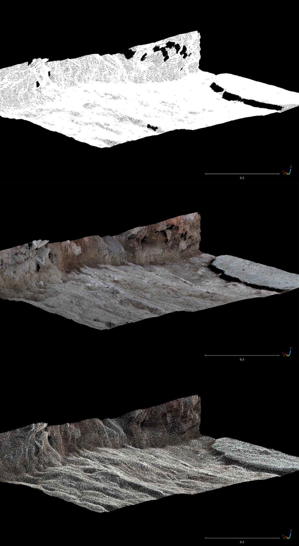
Figure 2
Resulting segmented point clouds, upper: Artec Leo, center: Nikon D5300, lower: iPhone.
Finally, orthophotos were generated for the assessment on color quality in QGIS (QGIS 2025). Orthophotos were generated for the photogrammetric capture in Metashape. As the iPhone app and Artec Studio do not allow orthophoto generation, the models exported from CloudCompare were imported in Blender using the BlenderGIS add-on (Blender GIS 2025), allowing preservation of their geolocation. The Blender GIS add-on uses an orthographic camera positioned above the georeferenced scanned surface. Along with the rendered image from this camera, a world (WLD) file is produced which contains the corner coordinates of the orthographic image. Based on the resulting 3D meshes in CloudCompare and orthophotos in QGIS, the quality evaluation presented below has been executed.
Comparison
Capture and processing times
Tables 2 and 6 include details on capturing and processing times. Capturing times for the Artec Leo and iPhone were equal and took about two minutes. The photogrammetric capture with the Nikon D5300 took significantly more time with 15 minutes. The processing times of the Nikon D5300 and Artec Leo data were significantly longer than those from the iPhone, respectively 62 and 30 minutes, also clearly reflected in the output data sizes (Table 6).
Table 6
Comparison of data processing details.
| DEVICE | PROCESSING SOFTWARE | PROCESSING TIMES | GEOREFERENCING | RESULT |
|---|---|---|---|---|
| iPhone | polyCam | 2 min | Targets, DGPS, CloudCompare | Pointcloud: 3,051,240 points Mesh: 157,668 polygons Texture resolution: 4096 × 4096 No. of textures: 1 |
| Nikon D5300 | Agisoft Metashape | 62 min | Targets, DGPS, Metashape | Pointcloud: 88,958,243 points Mesh: 2,799,653 polygons Texture resolution: 8192 × 8192 No. of textures: 1 |
| Artec Leo | Artec Studio | Ca. 30 min | Targets, DGPS, CloudCompare | Pointcloud: 6,011,060 points Mesh: 11,964,597 polygons Texture resolution: 8192 × 8192 No. of textures: 1 |
Geometrical analysis
The geometrical analysis of the clouds, that from this point on will be referred to as LiDAR (iPhone LiDAR), PG (Nikon D5300 photogrammetry), and SL (Artec Leo Structured Light) clouds, will start with an absolute accuracy comparison using the CTRs. Subsequently, they will be compared for relative accuracy comparison and volumetrics (cf. Paukkonen 2023).
CTR comparison
The import of the transformed CTR points in CloudCompare was checked on an individual point basis. The CTR points, as well as the GPCs, all deviate slightly in all the various meshes. These deviations are not constant but vary in direction and amount. As can be seen for the targets (Figure 3), they are positioned under or above the mesh, with deviations between 3 and 6 mm. The highest deviations are found in the z-values. Given this variability, the most likely origin of these inaccuracies is the average accuracy of the dGPS system, where such deviations fall within the expected error range. As such, for the quantitative analysis of the CTR points with the three clouds, a general inaccuracy with the reported values must be considered. Note that for all meshes, the same GPCs were used. The deviation of the georeferencing is therefore the same across the dataset.
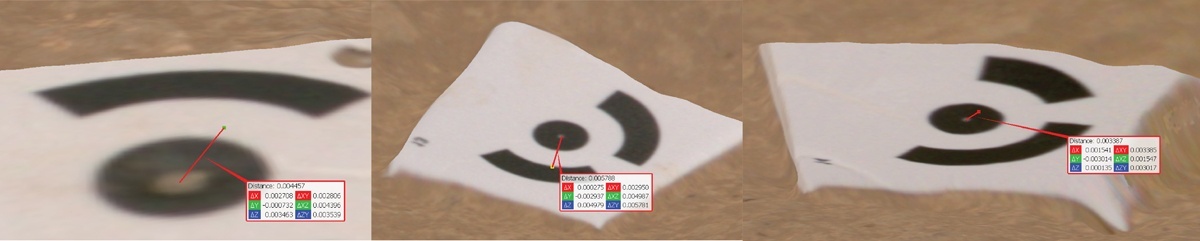
Figure 3
Comparison of GCP coordinates with locations on the SL mesh, left: target 12 above mesh, middle: target 13 under mesh, right: target 14 just under mesh.
The CTR comparison in CloudCompare was done with a subset of 10 CTRs, that were included into the extent of the point cloud segments. With the Compute cloud/cloud distance tool, taking the point clouds as reference, CloudCompare returns the distance statistics between the CTRs and the closest point in the point clouds.
As is clear from the table and graphs, the mean distances remain quite small for all techniques, with the PG cloud being the most accurate and the SL cloud following closely, albeit with a slightly higher standard deviation and maximum deviation (Table 7, Figure 4). The LiDAR cloud had a higher mean error, 9 mm, with a standard deviation similar to the PG cloud and a maximum like the SL cloud.
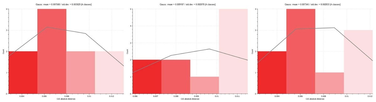
Figure 4
Distance deviation distributions of control points versus the different 3D capture techniques. Left: CTR vs SL cloud, center: CTR vs LiDAR cloud, right: CTR vs PG cloud.
Cloud-to-cloud comparison
The three clouds have also been directly compared using the same approach. As there are some parts where the clouds do not completely overlap (for example due to small holes in the clouds where data was insufficiently captured due to obfuscation, see below), the maximum error is relatively large compared to the CTR and cloud comparison (Table 8, Figure 5). There is no spatial patterning that suggests any systematic error (e.g., towards the edges of the area).
Table 8
Cloud to Cloud distances of LiDAR, PG, and SL clouds (N = >1.000.000).
| METRIC | LIDAR vs SL CLOUD | PG vs SL CLOUD | LIDAR vs PG CLOUD |
|---|---|---|---|
| Mean | 1.9 mm | 0.7 mm | 1.4 mm |
| StDev | 1.6 mm | 0.5 mm | 1.2 mm |
| Max | 25 mm | 23 mm | 22 mm |
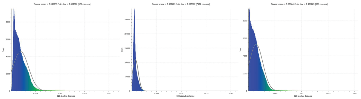
Figure 5
Distance deviation distributions of different combinations of 3D capture techniques. Left: LiDAR vs SL cloud, center: PG vs SL cloud, right: PG vs SL cloud.
From these comparisons, it can be observed that the distances between the PG cloud and the other clouds are the smallest, which falls neatly in line with the CTR vs clouds comparison, showing the best performance of the PG cloud. However, it must be emphasized that the overall distances are small throughout the clouds. For example, to consider the largest distances measured, the distance between the LiDAR and SL point cloud is 1.9 mm on average, with a standard deviation of 1.6 mm, which means that 68% of the measured distances deviate only between 0.3 mm and 3.5 mm.
Another option for looking at geometrical accuracy between the clouds is the multiscale model-to-model cloud comparison (M3C2) function (Barnhart & Crosby 2013) available in CloudCompare. This method looks at more general trends in the cloud surface, by creating geometrical cylinders following the trends in local regions of the cloud and defining normal vectors that summarize the mean orientation of those cylinders. These are then compared on mutual distances between the clouds (Figure 6). Because of the focus on more global trends in the data, this method is ideal for surfaces that deviate because of local irregularities or roughness that can be considered as noise. However, in case of low-noise clouds, this smoothing method can artificially reduce the cloud-to-cloud distance and should be used with caution. As the excavation’s surfaces are inherently rough, it would be wrong to consider this roughness as noise and should actually be used in the comparison. However, a reason to potentially use it may be in case of clouds with deviating numbers of points, where the thinner clouds have more holes which may cause the aforementioned distances between points and thus potential accuracy differences.
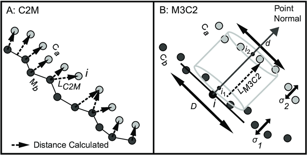
Figure 6
Illustration of the M3C2 cloud distance comparison method (Barnhart & Crosby 2013).
Assessing this for the LiDAR vs SL cloud comparison, it is clear that the smoothing effect indeed reduces the error, halving the mean error and significantly lowering the maximum error (Table 9, Figure 7). The latter is to be expected as the method will greatly reduce the effect of outliers. However, if we compare this to a LiDAR point cloud that has been densified by extracting more points from the mesh, the results are very similar to the direct cloud to cloud comparison above (Table 9, Figure 7). As such, the M3C2 comparison probably artificially removes deviations between the two clouds, and the results should in this case not be considered superior to the cloud-to-cloud distance computation.
Table 9
M3C2 comparison between LiDAR and SL clouds, cloud to cloud comparison of densified LiDAR and SL clouds (N = >1.000.000).
| METRIC | LIDAR vs SL CLOUD M3C2 | DENSIFIED LIDAR vs SL CLOUD |
|---|---|---|
| Mean | 0.8 mm | 1.9 mm |
| StDev | 1.5 mm | 1.6 mm |
| Max | 3.5 mm | 24 mm |
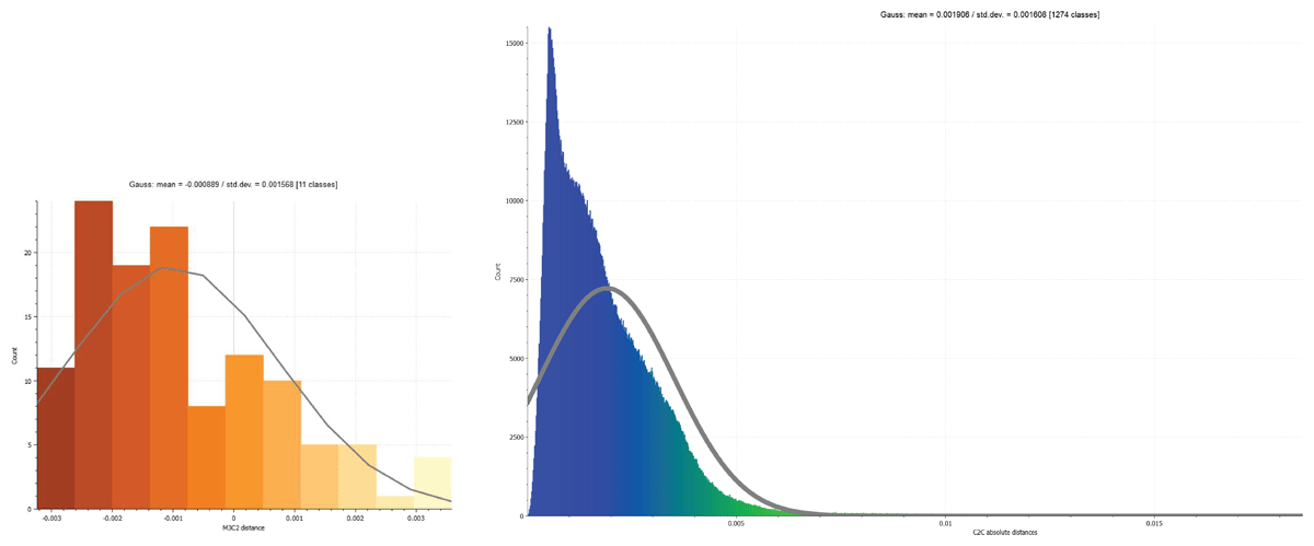
Figure 7
Assessment of the effect of computation method on cloud to cloud distances. The graphs display the distance distributions of LiDAR vs SL. Left: M3C2 computation method. Right: C2C computation method.
Volume comparison
Although the measured distances between the clouds are small, it remains relevant to understand to what degree this can result in local discrepancies in volume, that could ultimately be affecting soil quantity or find density calculations for example. In order to evaluate this effectively, a smaller section of the point clouds was extracted containing an irregular excavation surface (Figure 8). For volume comparisons, CloudCompare offers a 2.5D volume tool. The resulting volume discrepancies are negligible. Whereas at one very local spot there is a ca. 1.6 cm height difference (Figure 9), overall, all comparisons the average difference is below 0.000 cubic mm (Table 10).
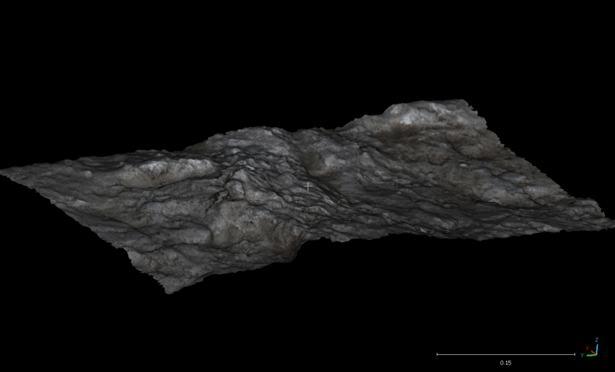
Figure 8
Extracted segment used for volume comparison (PG mesh).
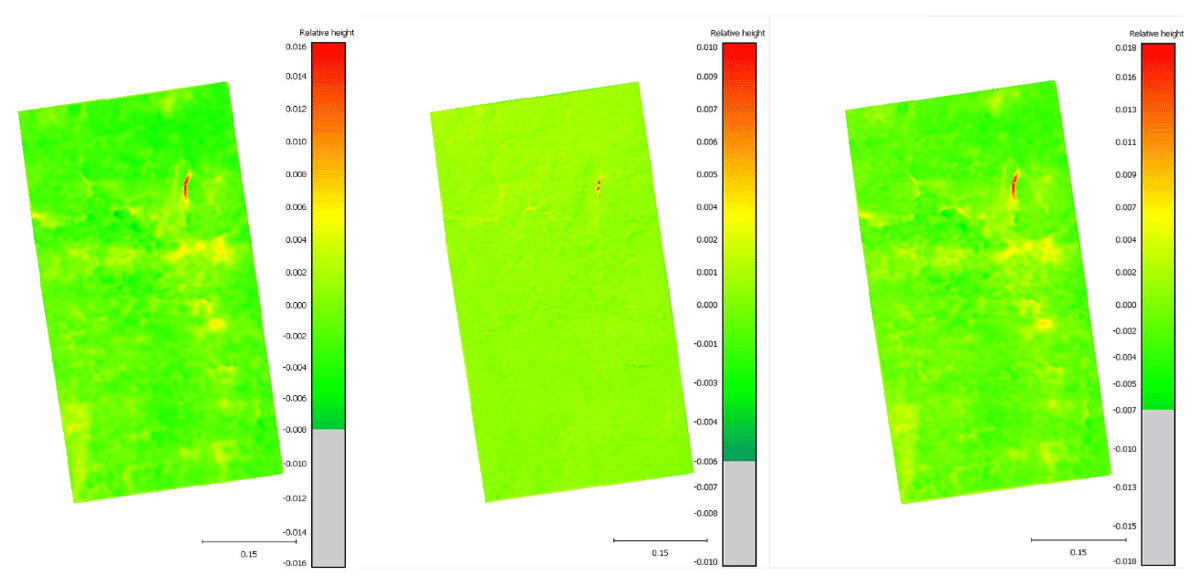
Figure 9
Volume comparisons. Left: SL vs LiDAR cloud, center: SL vs PG cloud, right: PG vs LiDAR cloud.
Texture analysis
The photographic textures are an important aspect of 3D documentation, as it determines the ability of the observer to interpret color and fine details otherwise not visible in the geometric surface model. Since the primary use of these textures is the interpretation of features by a human observer, their quality has been assessed and compared subjectively by visual analysis.
Comparing the textures, the color differences are striking (Figure 10). The SL texture has a rather particular creamy brown hue over it. As the Artec Leo uses flash photographic capture, the most likely explanation for this is that it uses a preset white balance based on the color temperature of this type of light. As the sun interferes significantly with the captures, the colors are shifted using the inaccurate white balance setting. No custom white balance setting is available on this device. In addition, due to this flash, shaded areas are significantly lit, producing less contrast in the texture. The LiDAR texture appears a bit overexposed, which may be because of automatic exposure settings (possibly a metering mode) in the PolyCam app. The PG texture reproduces the natural colors the best, which is to be expected from a decent DSLR camera. It does not exhibit the problems present in the SL and LiDAR textures, and has more contrast. Even uncalibrated, the hues of this camera best resemble the colors observed under the light conditions at capturing time. Of course, because the camera can capture in a raw image format, subsequent color calibration can further improve this. A downside of both the Artec LEO and the iPhone is they instead do not allow for color calibration, nor for custom white balance settings.
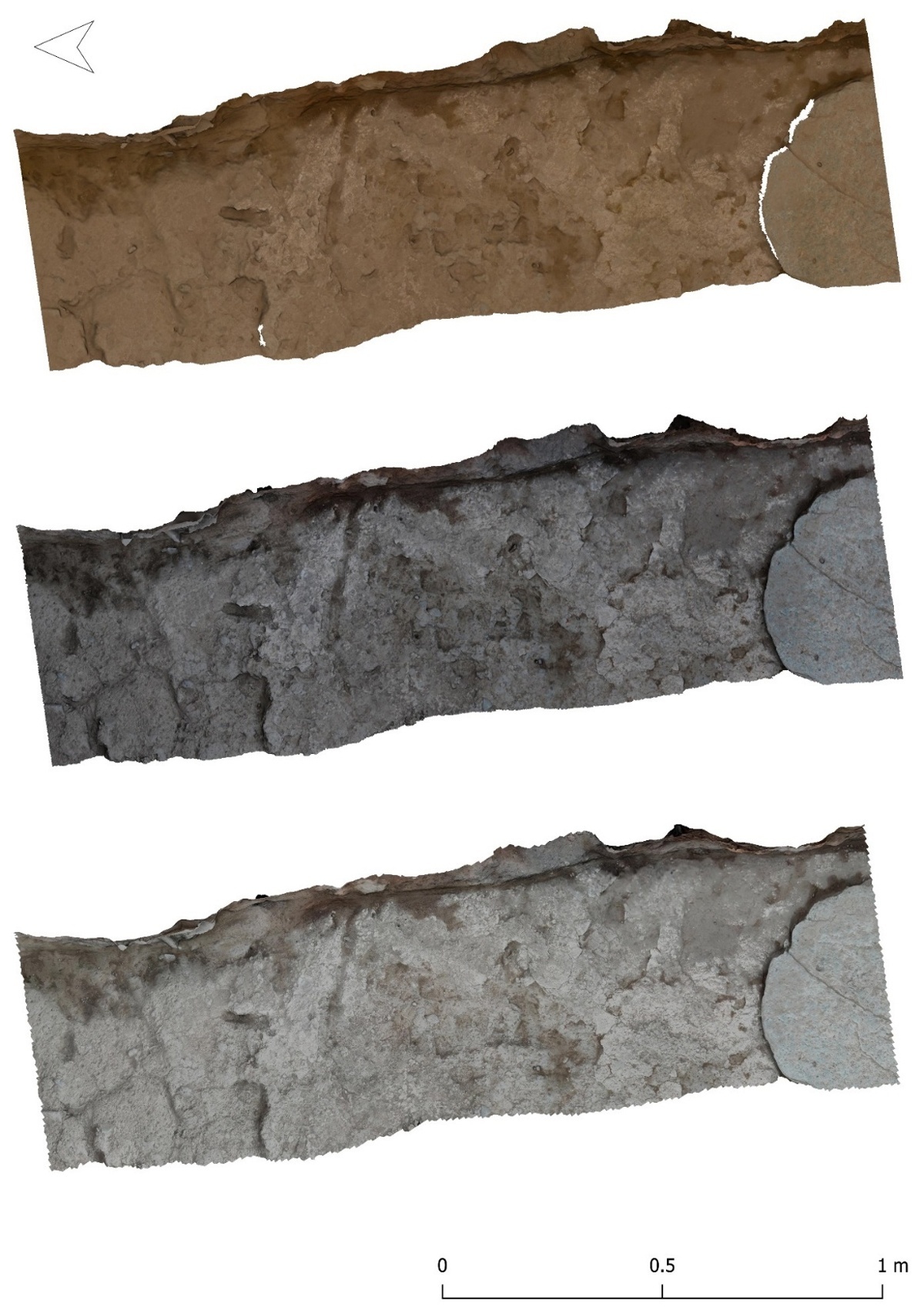
Figure 10
Texture comparisons. Upper: SL texture, center: PG texture, lower: LiDAR texture.
Zooming in on details of the textures, it is clear that the resolution is quite sufficient for archaeological excavation documentation (Figure 11). Also, the details can be seen to overlap nicely, with just the SL texture lacking a bit of visual clarity due to the aforementioned color shift of the texture. The white dots are two dGPS control points. Comparing their position relative to other features the LiDAR model shows slight deviations, possibly indicating that the surface reconstruction of PolyCam is slightly less accurate.
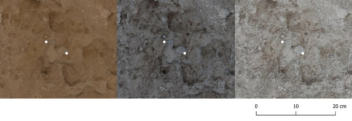
Figure 11
Texture comparisons. Left: SL texture, center: PG texture, right: LiDAR texture. White dots are CTRs.
Capture ergonomics and user friendliness
All three data capture methods exhibit a high degree of mobility, thereby enhancing their adaptability within excavation contexts. From an ergonomic perspective, both the iPhone and the Nikon camera are relatively lightweight, facilitating ease of positioning. Furthermore, the Osmo gimbal significantly enhances the smoothness of data capture operations as it supports rotating the iPhone automatically. In contrast, however, while the Artec Leo is designed for ease of handling and operation, its relatively large size can make it difficult to get into tight corners, which may be the cause for incomplete coverage and data gaps (Figure 12). In addition, its higher weight results in fatigue during prolonged data capture sessions.
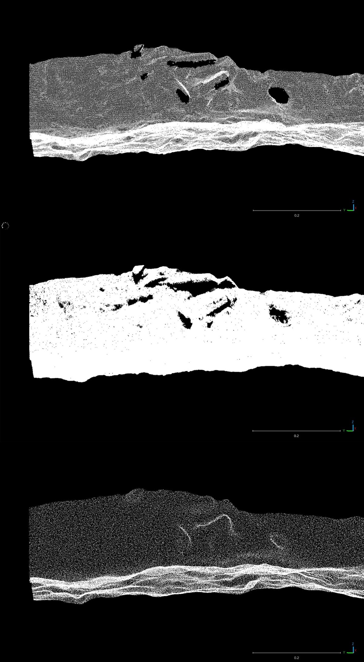
Figure 12
Resulting segmented point clouds of SL (upper), PG (middle), and LiDAR (lower) clouds, highlighting the differences in point density and data coverage in hard to reach areas.
Considering usability, the Artec Leo and the iPhone have distinct advantages, namely a model preview for the former, and on the spot processing for the latter, allowing direct assessment of the quality of the scans. As such, the data capture can immediately be checked on quality, and a rescan is possible if it is plausible that a better result can be attained. Photogrammetry, however, is more complex in the field, and quality control can only be done by subsequent processing and therefore takes more time.
Although the geometrical analysis showed a very high accuracy of the scans, there are still some gaps in the different clouds, mainly featuring with the SL and PG clouds. These occur at the locations where sherds protrude from the profile. As mentioned due to the ergonomics of the Artec Leo, it is very hard to scan the underside of protruding features close to the excavation surface. Even though the Nikon D5300 is smaller, it is still too large to properly capture some of these hard-to-reach areas. The iPhone however is smaller and more flexible, resulting in more complete coverage. However, it is still surprising that the LiDAR cloud does not feature any gaps at all, which is difficult to accept as also for the iPhone some areas were hard or impossible to cover properly. This suggests that the PolyCam software artificially closes these holes using interpolation algorithms.
Summary of the comparisons
Based on these comparisons, a short summary can be made of their relative qualities in this context. All three devices produce geometrically very good models, both in terms of measured distances between clouds, and in terms of the comparison of captured volumes. There are some inaccuracies, but these are mostly negligible for the process of archaeological excavation and documentation. Texture-wise there are some more pronounced differences, with a clear drawback of the Artec Leo for outside capture, rendering suboptimal colors and contrast. The PolyCam app on the iPhone tends to slightly overexpose but still produces very decent colors and contrasts. Overall, photogrammetry appears to work best, both for geometry, albeit with minute differences, as well as for texture quality, which is more significant. Considering the potential occurrence of gaps in the cloud due to occlusion as a result of complex 3D topography in relation to accessible scanning angles, the iPhone is probably the most effective one, especially in comparison to the Artec Leo, although it is still unclear to what degree interpolation may have closed some gaps in the resulting clouds. In terms of ergonomics and usability, the Artec Leo and the iPhone data capture depend less on skill level than photogrammetry and allow for a relatively quick data quality assessment. This likely results in a more solid data capture process in the case of less experienced field teams responsible for the 3D documentation. The iPhone exhibits superior versatility in capturing various angles of a scanning target, thereby minimizing the likelihood of occlusion in the resultant models. Additionally, while the duration of data acquisition in the field is comparably consistent across all three techniques, the processing times for the data exhibit significant variation. Specifically, photogrammetry requires the most extensive processing time, which may become a substantial factor when dealing with large areas.
Discussion of application contexts
In the end, as discussed in the introduction, the integration of new technology must be a well-considered choice where costs, available resources, output criteria, flexibility, etc., are all part of the equation. Although photogrammetry outperformed the other two techniques, mainly on texture quality, it still also requires the most expertise in the field and most processing time, and as a total package therefore constitutes a considerable investment, which can be a problem for projects with modest resources. It must be acknowledged, however, that real-time cloud-based computing solutions will soon likely provide a way for quick quality assessment with photogrammetry as well. It is nevertheless interesting that the iPhone in this specific context performed quite impressively, with a good geometrical accuracy and reasonable texture quality. Given its relatively low-cost, ease of use, speed, and flexibility, the iPhone can absolutely be an option to consider for projects running on low budgets, especially if the 3D documentation is considered as a ‘nice-to-have’ extra layer of data and the slightly less geometrical accuracy is not of fundamental importance.
However, other considerations must be included for a robust decision on using a system such as the Apple 15 pro LiDAR. Since the specifications for the LiDAR sensor have not been made public, it is, as mentioned earlier, a black-box technology. This means that there is no transparency as to the exact hardware and software mechanics of the technology, among other things hindering a fully FAIR approach to data production. In addition, there is the lurking danger of a project becoming too platform dependent. Although the same can be said about more producers of hardware and software solutions as a closed source interdependent ecosystem such as Artec, that technology and its producer could be expected to be a reasonably stable factor. However, in case of the iPhone, what if Apple decides, just as Samsung did earlier, to cancel the development line of iPhone-based LiDAR (Nogee 2021)? This would have an impact on long-term support and thus sustainability of an iPhone-based workflow. And indeed, an analysis of durability of the iPhone-based workflow has not been incorporated in the test. Although these are instruments that are optimized for outdoor use, it is yet unknown what the manufacturing quality of the LiDAR sensor is, and how that may degrade over time. As for workflow integration, mainly photogrammetry will have most impact on documentation workflows during fieldwork, as it takes more time for recording and processing and does not provide direct results, which has potential implications for the disruption of the excavation and quality control.
Conclusions and future prospects
In this paper, we have examined the comparative performance of three different 3D data capture technologies in the context of archaeological excavation documentation. Based on rigorous analysis and evaluation, we have shown that each of these devices—namely the Artec Leo, the iPhone LiDAR using the PolyCam app, and traditional photogrammetry—offers unique advantages and disadvantages. Our findings indicate that, while all three methods produce geometrically sound models, there are notable differences in texture quality, usability, and overall practicality in field settings. The results of this paper should not be taken as indicative for all potential application contexts of these technologies. For example, SL scanning is scale-dependent and can produce different quality results for considerably smaller or larger objects. Also, scanning distances are much more limited in comparison to photogrammetry. On the other hand, the problem with the color of the SL scans is much less of an issue in inside conditions. The performance of the iPhone LiDAR lacks extensive assessment with regards to different archaeological conditions. It is interesting that results have been found to be quite diverging in different contexts (cf. Paukkonen 2023). Also, it needs to be acknowledged that the iPhone LiDAR and PolyCam are likely to have been improved since 2023, which could result in different results in similar contexts when tested again. As such, it is important to repeat evaluations such as presented in this paper in different contexts to get a full picture of their relative performance.
Acknowledgements
This research has been conducted within the framework of the Halos Archaeological Project, associated with the Amsterdam Centre for Ancient Studies and Archaeology. The authors extend their gratitude to Project Director Vladimir Stissi for his sustained support and engagement throughout the duration of this project. Additionally, the contributions of Mikko Kriek, Mason Scholte, and Markus Stoffer, who played integral roles in the practical technological development and execution of the fieldwork, are acknowledged with appreciation. Special thanks are also due to the Director and staff of the Ephorate of Antiquities of Magnesia, as well as the Netherlands Institute in Athens, along with the local communities of Amaliapolis, Platanos, and Almyros, whose cooperation was essential to the success of this study. It is noteworthy that no external funding was utilized for any aspect of this research.