
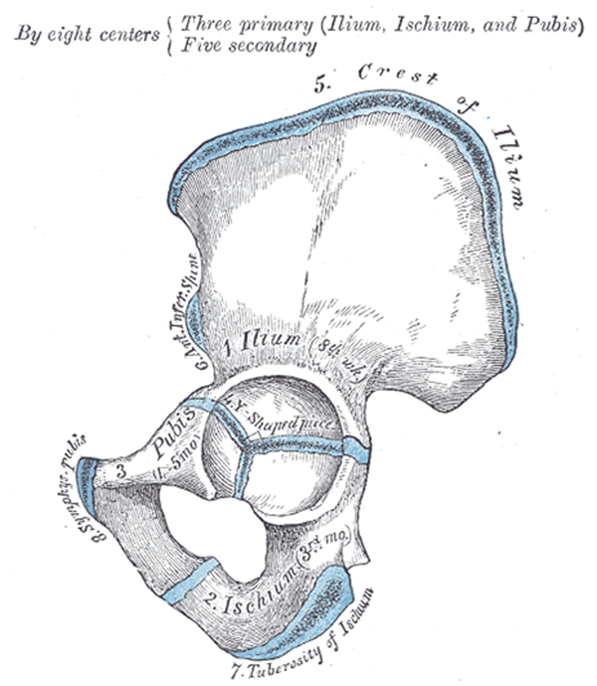
Figure 1
Modules of the os coxae (lateral view of the left side). The ilium, ischium and pubis are illustrated and, in light blue, their secondary ossification centres and the joints which fuse in maturity (Gray 1918: 238).
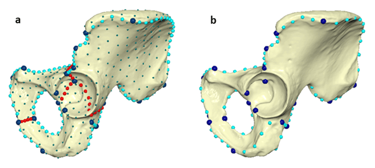
Figure 2
Os coxae digitisation templates created in Viewbox 4. The first template (a) substantially over-sampled the os coxae with coordinate points located at landmarks (dark blue), semi-landmarks along curves (light blue at extremal borders and red at borders between modules) and surface semi-landmarks (green). The revised template (b) contained fewer coordinate points and included landmarks (dark blue) and semi-landmarks along extremal borders (light blue). The final template is available at: https://doi.org/10.15131/shef.data.25498276) (Wigley and Blackwell 2024).
Table 1
The levels of ‘missingness’ introduced into simulated datasets.
| ‘MISSINGNESS’ | CONFIGURATIONS AFFECTED | VOLUME OF NAS IN DATASET | SIMULATED SCENARIO |
|---|---|---|---|
| Low | 25% | 10% | Small patches of NAs simulating a reasonably complete assemblage with minor cortical erosion |
| High | 75% | 30% | Large patches of NAs mimicking assemblages affected by post-mortem disturbance and severe fragmentation |
| Diffuse | 100% | 20% | Patches of NAs reflecting an assemblage deposited in a substrate incompatible with cortical preservation and affected by factors promoting moderate fragmentation |
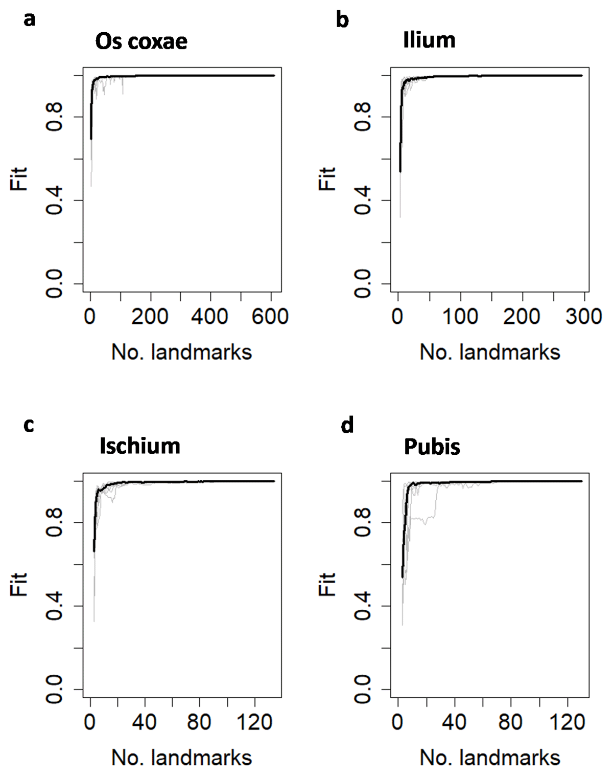
Figure 3
LaSEC sampling results. Plots illustrate the ‘fit’ between full and sampled configurations achieved by each of the ten iterations of sampling (grey lines) as well as the overall median fit (black line) for the whole os coxae (a), ilium (b), ischium (c) and pubis (d).
Table 2
Procrustes ANOVA to investigate factors affecting os coxae morphology. Significance determined through RRPP with 1000 permutations.
| EFFECTS | DF | SS | MS | R2 | F | P |
|---|---|---|---|---|---|---|
| site | 1 | 0.0135 | 0.0135 | 0.0699 | 2.1756 | 0.004 |
| sex | 1 | 0.0183 | 0.0183 | 0.0947 | 2.9475 | 0.001 |
| residuals | 26 | 0.1612 | 0.0062 | 0.8354 | ||
| Total | 28 | 0.1929 |
Table 3
Numerical summary of the distances between consensus configurations from datasets with imputed coordinate points and the consensus of the observed data.
| MISSING VALUES | ALIGNMENT | METHOD | MINIMA | 1ST QUARTILE | MEDIAN | MEAN | 3RD QUARTILE | MAXIMA |
|---|---|---|---|---|---|---|---|---|
| Low | unaligned | RF | 0.009452 | 0.012047 | 0.013577 | 0.013664 | 0.014965 | 0.021430 |
| TPS | 0.001209 | 0.001387 | 0.001498 | 0.001519 | 0.001642 | 0.001906 | ||
| aligned | RF | 0.001593 | 0.002149 | 0.002320 | 0.002307 | 0.002465 | 0.002744 | |
| TPS | 0.001214 | 0.001390 | 0.001503 | 0.001521 | 0.001639 | 0.001909 | ||
| High | unaligned | RF | 0.050420 | 0.066490 | 0.073960 | 0.074880 | 0.083280 | 0.100650 |
| TPS | 0.005311 | 0.006565 | 0.007005 | 0.007046 | 0.007520 | 0.009426 | ||
| aligned | RF | 0.005585 | 0.007205 | 0.007787 | 0.007798 | 0.008345 | 0.009446 | |
| TPS | 0.005228 | 0.006464 | 0.006908 | 0.006940 | 0.007365 | 0.009446 | ||
| Diffuse | unaligned | RF | 0.047070 | 0.062250 | 0.066290 | 0.067840 | 0.073940 | 0.087280 |
| TPS | 0.006112 | 0.006854 | 0.007383 | 0.007320 | 0.007717 | 0.008631 | ||
| aligned | RF | 0.005973 | 0.006655 | 0.006973 | 0.007091 | 0.007364 | 0.009446 | |
| TPS | 0.006196 | 0.006921 | 0.007506 | 0.007442 | 0.007839 | 0.008845 |
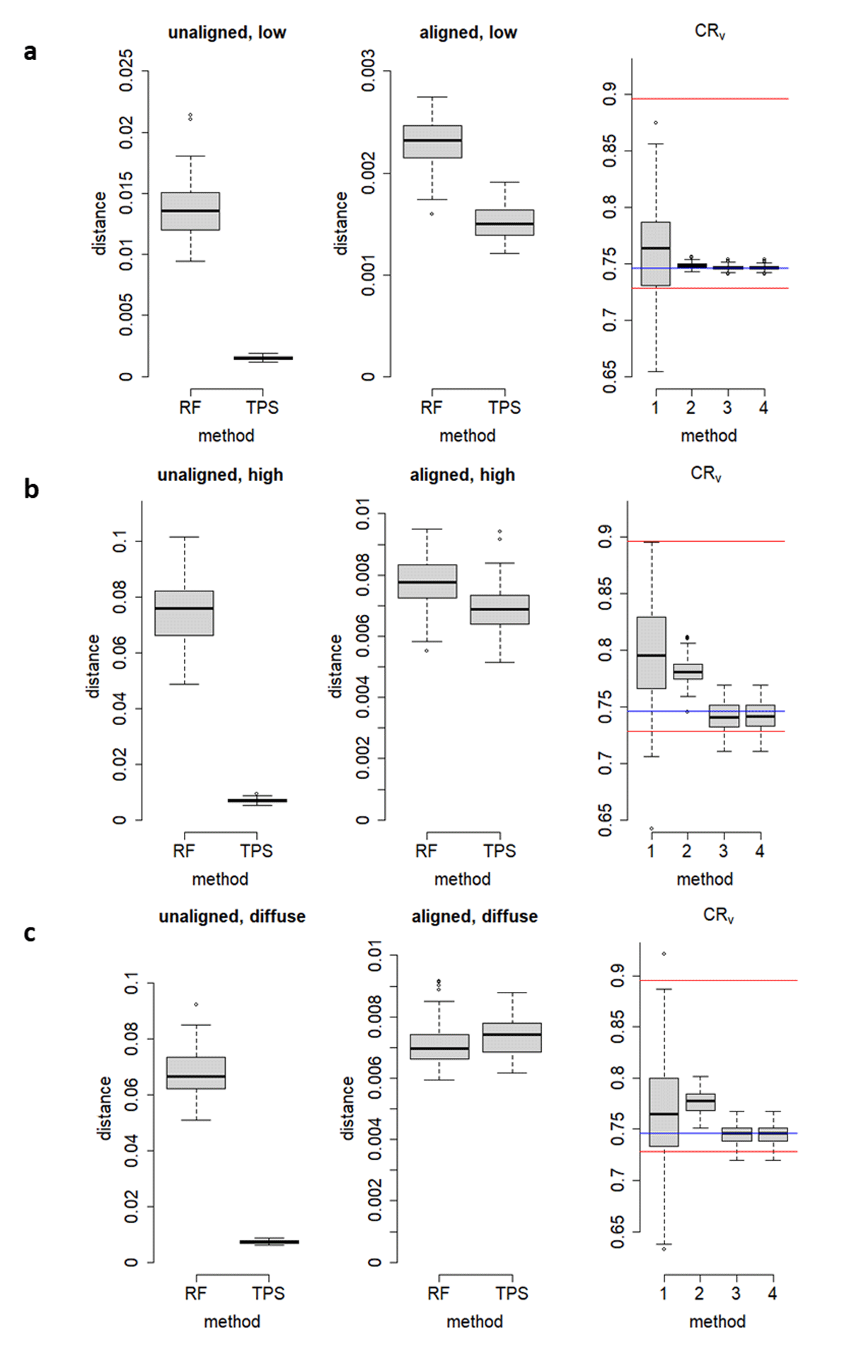
Figure 4
Boxplots evaluating the performanace of imputation methods. These represent the distance between the observed consensus configuration and the consensus configurations of unaligned and Procrustes-aligned simulated datasets with ‘low’ (a), ‘high’ (b) and ‘diffuse’ (c) missing data after NAs had been filled by either RF or TPS imputation. On the righthand, the CRν coefficients associated with unaligned RF (1), aligned RF (2), unaligned TPS (3) and aligned TPS datasets (4) are also contrasted to the observed coefficient (blue line) and the upper and lower 95% CIs suggested by boostrapping (red lines).
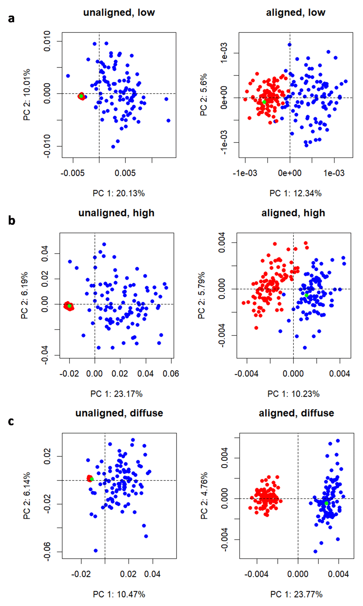
Figure 5
PCA visualisations. Plots illustrate the relationship between the observed consensus configuration (green) and consensus configurations associated with aligned and unaligned datasets with ‘low’ (a), ‘high’ (b) and ‘diffuse’ (c) levels of missing values filled by RF (blue) and TPS (red) imputation.