
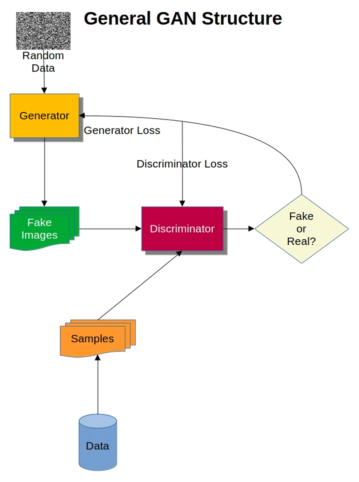
Figure 1
General structure and workflow of a basic ‘vanilla’ GAN showing the role of the generator and discriminator in generating ‘fake’ images and using real image data to compare with generated images.
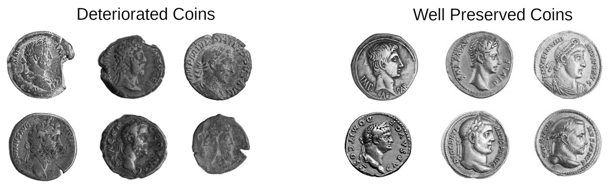
Figure 2
Example coins divided into deteriorated and well preserved coin categories (or ‘bad’ and ‘good’ coins) used to train our GAN. Others can be found in the supplementary data.
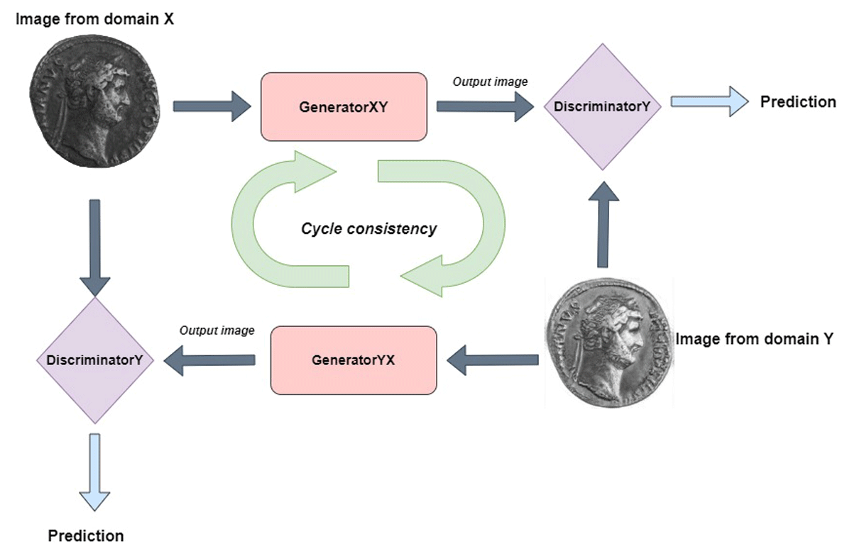
Figure 3
The CycleGAN-based approach applied in reconstructing coins.
Table 1
Relevant hyperparameters for the CycleGAN deployed.
| INPUT PARAMETER | VALUE |
|---|---|
| Epochs | 155 |
| Image Dimensions | 256 × 256 |
| Loss Function | Least Squares GAN |
| Patch Size | 196 × 196 |
| Batch Size | 1 |
| Initial Learning Rate | 0.0002 |
Table 2
Results (in percent) from the first test checking accuracy in distinguishing real and generated coins using 20 coins.
| EVALUATOR | ACCURATE IDENTIFICATION |
|---|---|
| Evaluator 1 | 35% |
| Evaluator 2 | 50% |
| Evaluator 3 | 45% |
| Evaluator 4 | 45% |
| Evaluator 5 | 55% |
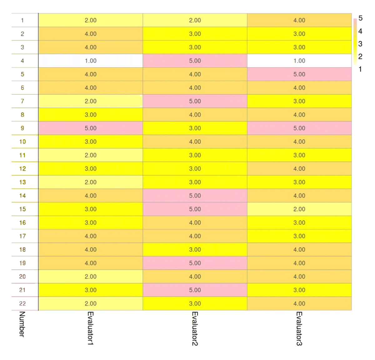
Figure 4
Second test performed showing respondent results evaluating reconstructions and checking for visual improvement quality (1–5; 1 reflects no improvement and 5 reflects excellent improvement).
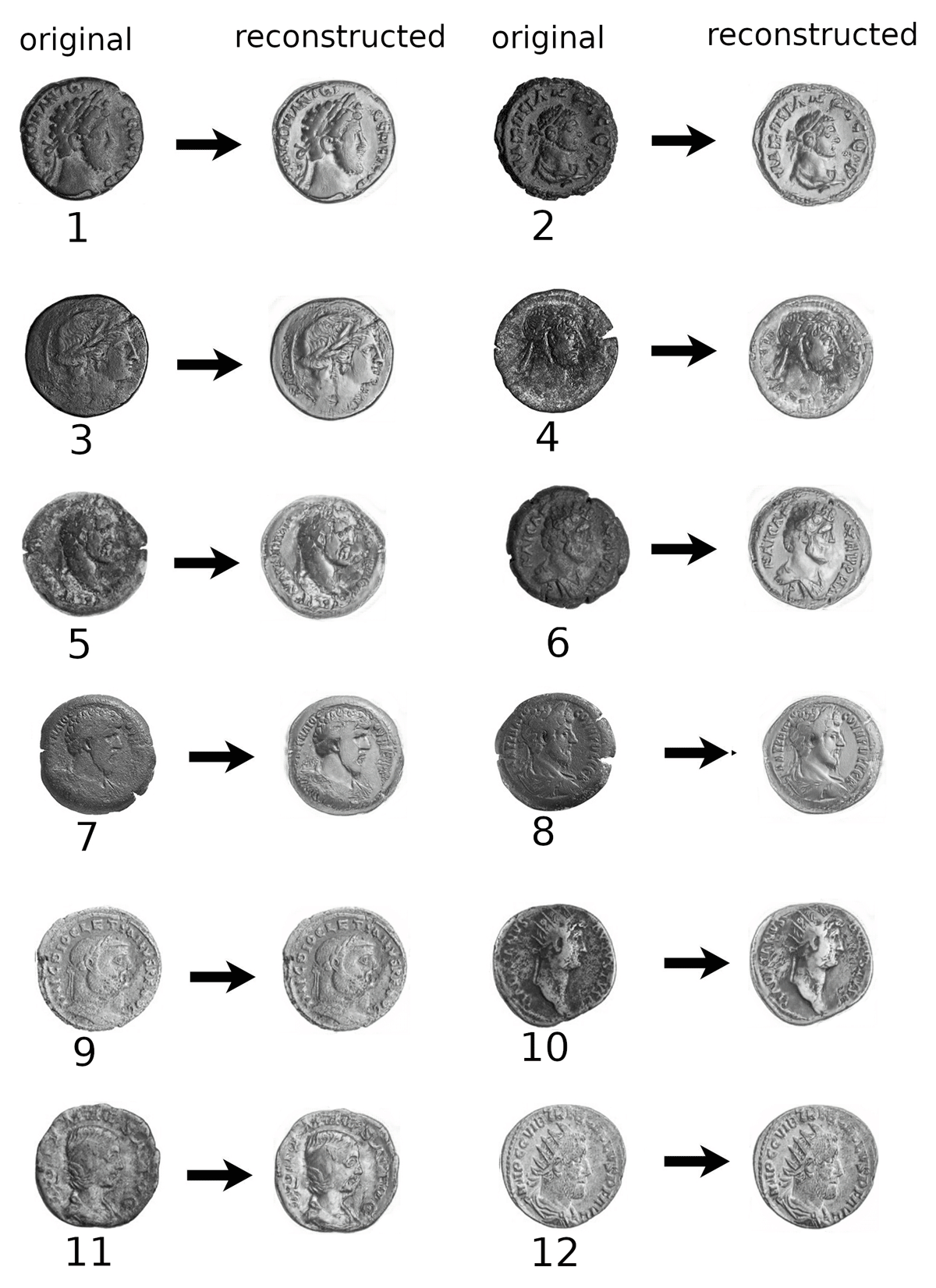
Figure 5
Example GAN reconstructions showing original (left) and reconstructed (right) Roman coins (obv.).
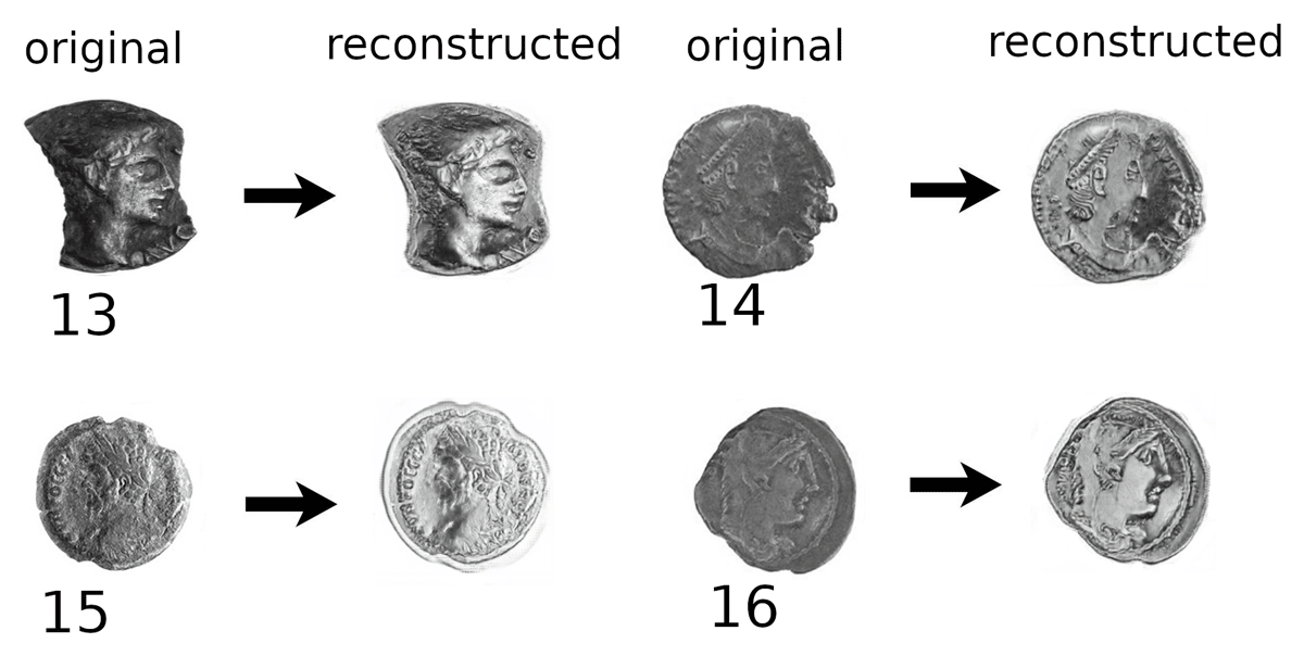
Figure 6
More heavily degraded real coins (left) and reconstructed (right) coins (obv.) using the CycleGAN. These examples highlight how the GAN addresses coins having 40% or more surface damage in cases.