
1. Coastal Proximity
The spatial analysis of coastal landscapes, or coastscapes, within archaeology tends to focus on vulnerability assessment in heritage management (Ashmore 2005; Reeder, Rick & Erlandson 2012; Hil 2020; Westley et al. 2023), the reconstruction of site palaeogeomorphology (Anzidei et al. 2011) or predictive site modelling (Jochim 2022).1 Considerably less prevalent are analyses of archaeological site coastal proximity and the effort of movement between site and the sea as a marker of the integration of the coastal zone into daily lives of past humans (Nuttall 2021a; 2021b; Roalkvam 2023). There has been a multitude of work on mobility and movement through space in archaeology and anthropology in recent years (Hammer 2014; Richards-Rissetto & Landau 2014; Verhagen, Nuninger & Groenhuijzen 2019) and Coastal Proximity Analysis (CPA) aligns with this tradition. CPA challenges and transcends absolute spatial and Euclidean models (Conolly & Lake 2006: 3) of the spatial relationship from site to coast, which fail to capture the nuanced and variegated impact of palaeotopography and the realities of bodily movement through that landscape. The association between human activity and coastal proximity does not, in itself, provide a causal relationship between coast and society. Rather, it presents a circumstance which can be further expounded upon, utilising cultural, topographical, and environmental contextual information. Its utility is in identifying periods of greater or lesser coastal proximity in settlement patterns. CPA supersedes modern spatial analytical indicators (e.g., Kiousopoulos 2008) which focus on the modern conceptualisation of the coast, with its modern associations, which are ultimately incompatible with ancient perspectives towards the sea.
In this delineated framework, this article turns attention to the effort or “cost” of movement between site and coast, operationalised using a Geographic Information System (GIS). Leveraging satellite imagery, Digital Elevation Models (DEMs) serve as digital representations of complex palaeotopographies. From this foundational layer, a CPA is conducted, the method of which is presented, before it is enacted in case studies focusing on prehistoric Greek settlement patterns on three Greek islands, Kea in the Cyclades, Kefalonia in the Ionian islands, and Kos in the Dodecanese (Figure 1). This new spatial analysis must be accessible and replicable, harnessing openly sourced data and a straightforward methodology. To this end, the current proposal engages the ‘least cost path’ function (LCP) within the open-source environment of QGIS (QGIS Development 2023), thereby generating an empirically grounded metric for the spatial interplay between locale and palaeocoastline. These paths do not serve as a suggestion for the exact routes taken by past people to the coast, who may have had a range of logical or cultural reasons to choose alternative and less efficient paths, and such prehistoric movement routes cannot be accurately determined due to the absence of records of these routes on the islands. Furthermore, verifying ethnographic routes through the islandscapes of these islands using traveller accounts is beyond the scope of this paper. The LCP analysis, therefore, serves solely as an index of coastal proximity, suggesting the fastest possible route.
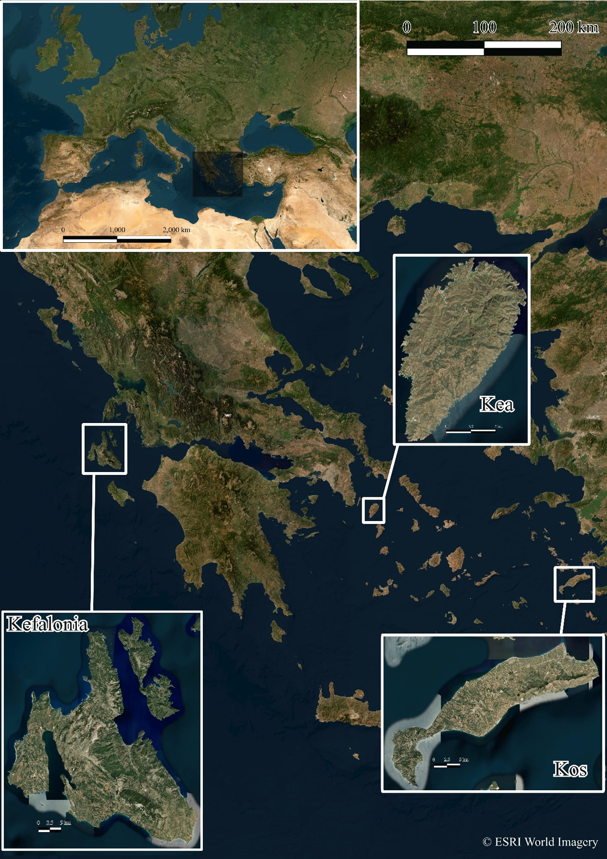
Figure 1
The areas of interest chosen for the application of Coastal Proximity Analysis.
2. Method
In alignment with the theoretical aims of this analysis, the methodological schema of CPA hinges upon an in-depth exploration of palaeolandscape morphology, thus necessitating a nuanced acknowledgment of the validity — or lack thereof — between contemporary topographical configurations and historical antecedents. This enables the researcher to gain a closer understanding of the environment past people could have encountered. The DEM selection is not a technicality but the bedrock upon which the GIS analysis is built. The EU-DEM dataset, verified through multiple quality assessments (Józsa, Fábián & Kovács 2014; Mouratidis, Karadimou & Ampatzidis 2017) and freely available, serves as the analytical crucible for the GIS enquiries presented here. It is, however, also acknowledged that more recent land use could have impacted the surface features of these rasters (Herzog & Yépez 2015; Lewis 2023: 17).
Simultaneously, we are confronted with the complexities of palaeoshorelines, accentuated by variables including sea level change, the localized impact of alluvial-colluvial episodes, seismic subsidence, and erosion processes. Sea levels have increased over time, though this is in tandem with oppositional processes, for example alluvial episodes that have the capability to expand the coastal area extent putting previously coastal settlements further inland (Kraft, Aschenbrenner & Rapp 1977), as well as seismic subsidence that can raise sites previously on the water line to several metres above sea level (Stiros & Blackman 2013). To mitigate these concerns, the analysis deploys digital bathymetric models (DBMs)—in this case, the publicly accessible EMODnet models—as instruments to estimate submerged topographies (EMODnet 2024). These DBMs are compiled and constructed though the combined effort of marine science projects, governmental departments and national hydrographic services. Before conducting the CPA, a DEM raster is created through the merging of topographic and bathymetric models. This reconstructed palaeolandscape is then projected onto an appropriate grid (EPGS: 2100/Greek Grid), to better lay the foundations for the LCP analysis. Within this framework, the ancient shoreline (for example “–6” from the DBM) is assigned an elevation value of “1,” while all other raster cells are scaled up based on the specific parameters of the analysis.
An initial key step involves depicting the palaeoshoreline as a series of points. This is done by extracting contours from the original DBM, using the GDAL ‘contour’ function (gdal:contour), selecting a desired sea level, such as “–6” (GDAL/OGR Contributors 2020). This function in QGIS generates a polyline that represents the ancient shoreline. To make this usable for the LCP function, the polyline must be converted to a dense series of points using the QGIS function ‘extract vertices’ (native:extractvertices). The output is a shapefile populated with points, delineating the palaeoshoreline for the period under study.
In GIS-based modelling of movement paths, the cost surface—a representation of the effort required to traverse the landscape—is crucial for evaluating different routes. This can be readily calculated using GDAL ‘slope’ analysis (gdal:slope), using Horn’s function as standard, which calculates slope in degrees of inclination. A particular challenge arises with slope rasters when encountering zero slope, as such cells misleadingly register as having no cost (Kantner 2012), even though distance is still being covered. A practical workaround is Tobler’s hiking function (Tobler 1993), which allocates a time-based cost for each degree of slope, though alternative formulations exist based on energy expenditure, rather than time cost (Herzog 2013; Verhagen, Nuninger & Groenhuijzen 2019). Incorporation of Tobler’s hiking function allows for a better estimation of the time spent on each path, humanising the analysis which otherwise results in a line with an assigned cost value. This function has been adopted in various LCP studies within the scope of archaeology (Kantner 2012; Phillips & Leckman 2012; Surface-Evans 2012; Lothrop et al. 2018; Seifried & Gardner 2019; Rosenswig & Martínez Tuñón 2020) and is included here to lend a more anthropocentric dimension to the spatial relationship between sites and coastlines. In QGIS, this can be achieved using the Raster calculator with the following formula (Tobler 1993: 2):
This formula uses the initial slope raster from the DEM as its basis. Given the DEM’s 30 m spatial resolution, this measure serves as the reference for the algorithm. The outcome is a time-cost raster, which informs the time-based output of the generated LCPs.
LCP analysis computes the most efficient route between two specified points within a GIS landscape. Frequently used in archaeological research (Herzog 2014), LCP has applications in various domains such as resource exploitation (Taliaferro, Schriever & Shackley 2010), site prediction modelling (Rogers, Collet & Lugon 2017), population movement (Gustas & Supernant 2019; Gowen & de Smet 2020), maritime movement (Gustas & Supernant 2017; Peterson 2022) and the study of ancient road networks (Diwan & Doumit 2017; Lewis 2021). Dijkstra’s algorithm (Dijkstra 1959) is commonly employed for LCP analysis and is the preferred algorithm of choice here. In QGIS, the LCP analysis can be carried out via the Least Cost Path plugin (FlowMap Group@SESS-PKU 2021). The benefit of the plugin is that it allows for batch processing of multiple LCPs, thereby enhancing time efficiency. The ‘cost raster’ layer utilises the Tobler’s hiking function cost-surface raster prepared earlier. The ‘start-point layer’ is the dataset of sites under analysis. The ‘iterate over this layer’ option should be activated, creating an individual LCP for each point in the dataset. For ‘endpoints,’ the previously generated palaeocoastline shapefile is used and the ‘Only connect with nearest end points’ option is enabled. This narrows down the analysis to the nearest end point for each site, avoiding unnecessary additional calculations. Post-analysis, individual shapefiles representing each LCP are consolidated into a composite shapefile using QGIS function ‘merge vector layers’ (native:mergevectorlayers). The ‘total cost’ for each LCP is indicated in the Attribute Table, which is originally tabulated in hours’ walking time (Figure 2). These values can be converted to minutes, by multiplying by 60 or by 3600 for seconds, enabling a more intuitive interpretation of the data (Figure 3). The end-value is the Coastal Proximity Value (CPV).

Figure 2
Least Cost Paths with time value generated using Tobler’s Hiking function.
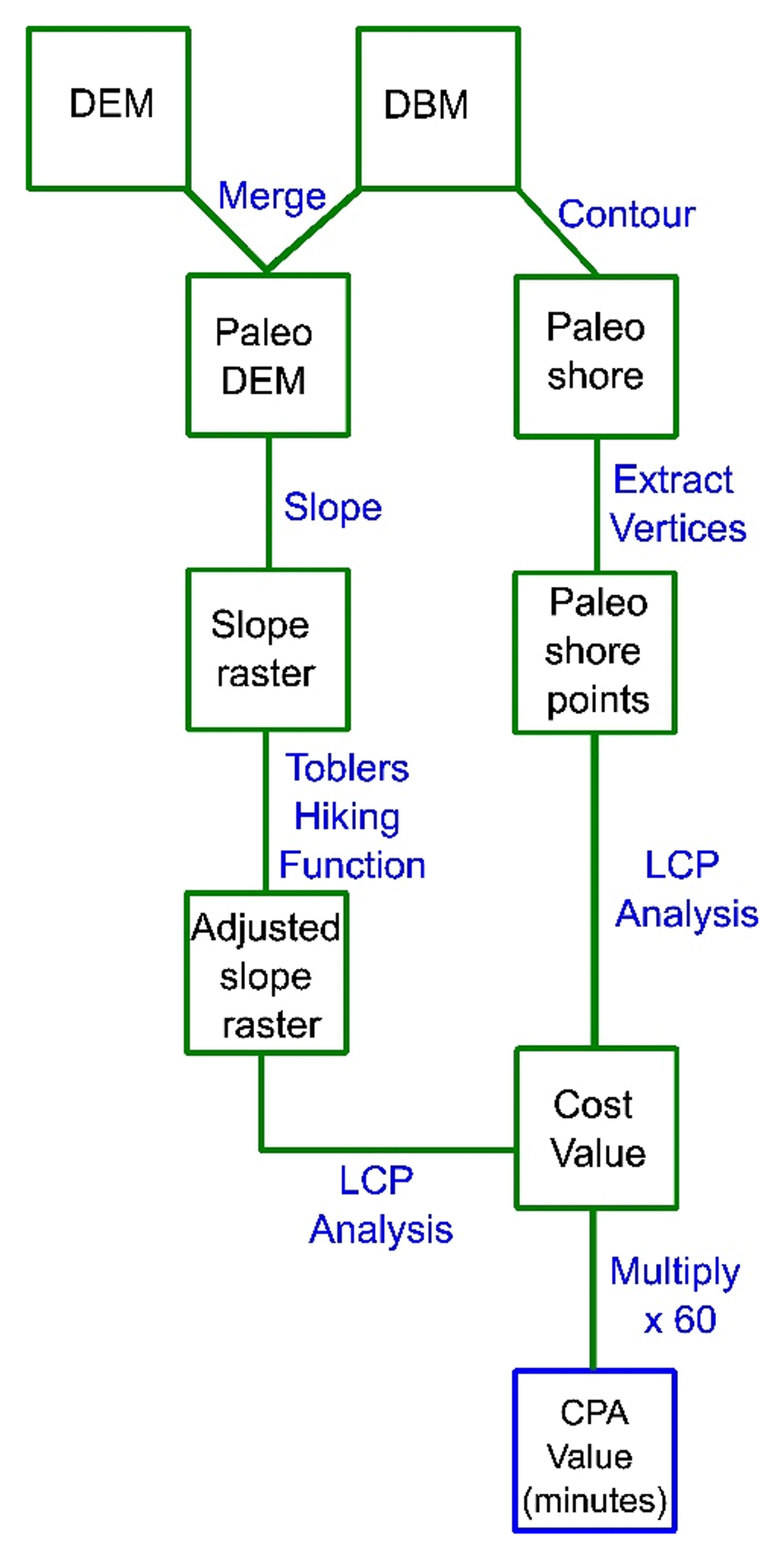
Figure 3
Workflow chart for the stages required for the Coastal Proximity Analysis.
The end goal of CPA is to quantify the temporal and spatial relationship between a specific location and the ancient shoreline, before interpretation of the social, economic, or practical reasons for coastal proximity. The framework is versatile, allowing for the integration of additional variables. For instance, viewshed analyses can be employed to assess the visibility of the sea from specific sites, thereby enriching the spatial data. Additionally, the geographical layout of a region can be analysed to determine its natural predisposition for coastal habitation, offering a more nuanced understanding of the area’s coastal proximity.
3. Case Study: Greek Islandscapes
The utility of any analytical approach is best measured by its effectiveness. In this case, a spectrum of prehistoric sites on Kea, Kefalonia and Kos (Figure 4), undergo the scrutiny of the above-delineated analytical framework. These islands have been chosen due to their extensive research histories, while each island represents one of the major island archipelagos of Greece. The defining feature, however, is that each has been subject to systematic fieldwalking surveys, the results of which are of a sufficient resolution to determine settlement patterns in differing chronological periods. The datasets on Kea derive from fieldwalking survey undertaken during the Northern Kea Archaeological Survey (Cherry, Davis & Mantzourani 1991) and the Northwestern Kea fieldwalking survey (Georgiou & Faraklas 1985). The data from Kefalonia is derived from the doctoral thesis of Souyoudzoglou-Haywood (1999) and the Livatho Valley Survey (Souyoudzoglou-Haywood 2008).2 The data on Kos is derived from the research undertaken by Halasarna Survey Project (Georgiadis 2012) and the Kos Archaeological Survey Project (Vitale et al. 2021). All three case studies encompass settlement patterns spanning from the LN to the terminal phase of the LBA (Table 1), which have been dated on the basis of surface ceramics and where undertaken, the excavation of the site. Employing this methodological framework allows for the nuanced tracing of an evolving relationship between sites and palaeocoastlines over various chronological periods on three different Greek islands.

Figure 4
Sites and places mentioned in the text.
Table 1
Chronological span of the case studies.
| RELATIVE CHRONOLOGY | ABSOLUTE CHRONOLOGY (BCE) |
|---|---|
| Late Neolithic (LN) | 5500–4500 |
| Final Neolithic (FN) | 4500–3100 |
| Early Bronze Age (EBA) | 3100–2000 |
| EB I | 3100–2700 |
| EB II early (EB IIA) | 2700–2400 |
| EB II late (EB IIB) | 2400–2200 |
| EB III | 2200–2000 |
| Middle Bronze Age (MBA) | 2000–1650 |
| MB I | 2000–1900 |
| MB II | 1900–1750 |
| MB III | 1750–1650 |
| Late Bronze Age (LBA) | 1650–1100 |
| LB I | 1650–1550 |
| LB II | 1550–1430 |
| LB IIIA | 1430–1300 |
| LB IIIB | 1300–1190 |
| LB IIIC | 1190–1100 |
The fundamental departure point for this analysis involves establishing the geomorphological parameters of these islands. For palaeosealevel, Lambeck’s seminal work on the Aegean (1995; 1996) indicates that an approximate depth of 5 metres below contemporary sea levels is applicable for the FN and EBA periods (Table 2), whilst a measurement of approximately 4 metres below present offers a reliable gauge for the MBA and LBA sea level. Alluvial deposits are reported in the larger valleys on Kea (Cherry, Davis & Mantzourani 1991: 58), though surface visibility in the coastal areas is good, proven by the identification of several ancient sites in these locations. Volcanic-related seismic uplift has been identified in central Kos (Dermitzakis, Kyriakopoulos & Ntrinia 2001: 30), though it is unclear how much of an impact this process had during the Holocene. Alluvial plains are almost entirely absent on Kefalonia (Souyoudzoglou-Haywood 1999: 4). In all three case-studies, no sealevel-related geomorphological investigations have been undertaken and so there are presently no known circumstances to indicate that the figures suggested by Lambeck are not applicable and it is unlikely that such changes would have drastically affected these estimates, which provide a more historically-relevant palaeocoastline estimate than present-day shorelines.
Table 2
Relative sea level difference to the present-day sea level.
| PERIOD | DEPTH BELOW PRESENT (M) |
|---|---|
| LN | –6 |
| FN–EBA | –5 |
| MBA–LBA | –4 |
The outcomes of the CPA are articulated in Table 3. The time values, presented in minutes, represent the median for all sites manifesting evidence of human activity within each respective phase. Before delving into an interpretation, several caveats merit attention. A portion of the sites bear only a nebulous chronological identification, categorised simply as ‘prehistoric’ or under broad time frames such as ‘Late Bronze Age’ (some 550 years in total), while other sites benefit from more precise chronological anchoring. The dataset (Appendix 1/Nuttall 2024) encompasses 229 sites in total, 89 on Kea (Figure 5), 57 on Kefalonia (Figure 6) and 83 on Kos (Figure 7). Some temporal spans, however, are represented by relatively few sites, thereby rendering median values for these periods less instructive. The geographic scope of the survey also imposes certain limitations and nuances on the results. The Kea and Kos survey areas are a patchwork of coastal and inland terrains; however, given these islands’ modest size relative to larger Mediterranean landmasses like Crete or Sicily, proximity to the coast emerges as a more prevalent feature in the dataset. The sea, in essence, is never truly beyond pedestrian reach anywhere on these islands. Kefalonia on the other hand, has a considerably different topography, as a larger island with taller mountains. What this analysis principally aims to elucidate then, is not so much remoteness from the coast as the frequency with which sites cluster along the immediate shoreline as opposed to a more inland positioning.
Table 3
Results of the Coastal Proximity Analysis, divided by island and chronological period. The ‘Median time-cost’ comes in minutes on foot.
| CHRONOLOGY | KEA | KOS | KEFALONIA | |||
|---|---|---|---|---|---|---|
| MEDIAN TIME-COST | COUNT | MEDIAN TIME-COST | COUNT | MEDIAN DISTANCE | COUNT | |
| LN/FN | 1.83 | 15 | 14.43 | 35 | 10.98 | 3 |
| EB I | 2.16 | 3 | 8.76 | 8 | NA | 1 |
| EB II early | 8.19 | 3 | 10.8 | 13 | NA | 1 |
| EB II late | 4.68 | 4 | 10.74 | 11 | NA | 1 |
| EB III | 9.18 | 2 | 6.78 | 11 | NA | 0 |
| EBA | 4.38 | 20 | 13.62 | 55 | 30.18 | 11 |
| MBA | 5.49 | 22 | 9.27 | 8 | 30.18 | 11 |
| LBA | 5.52 | 49 | 15.42 | 28 | 30.6 | 9 |
| LB I | 6.48 | 15 | 4.17 | 2 | NA | 1 |
| LB II | 7.05 | 14 | 4.17 | 2 | NA | 2 |
| LB III | 7.32 | 5 | 15.15 | 12 | 22.38 | 21 |

Figure 5
Kea and the distribution of sites included in this study.
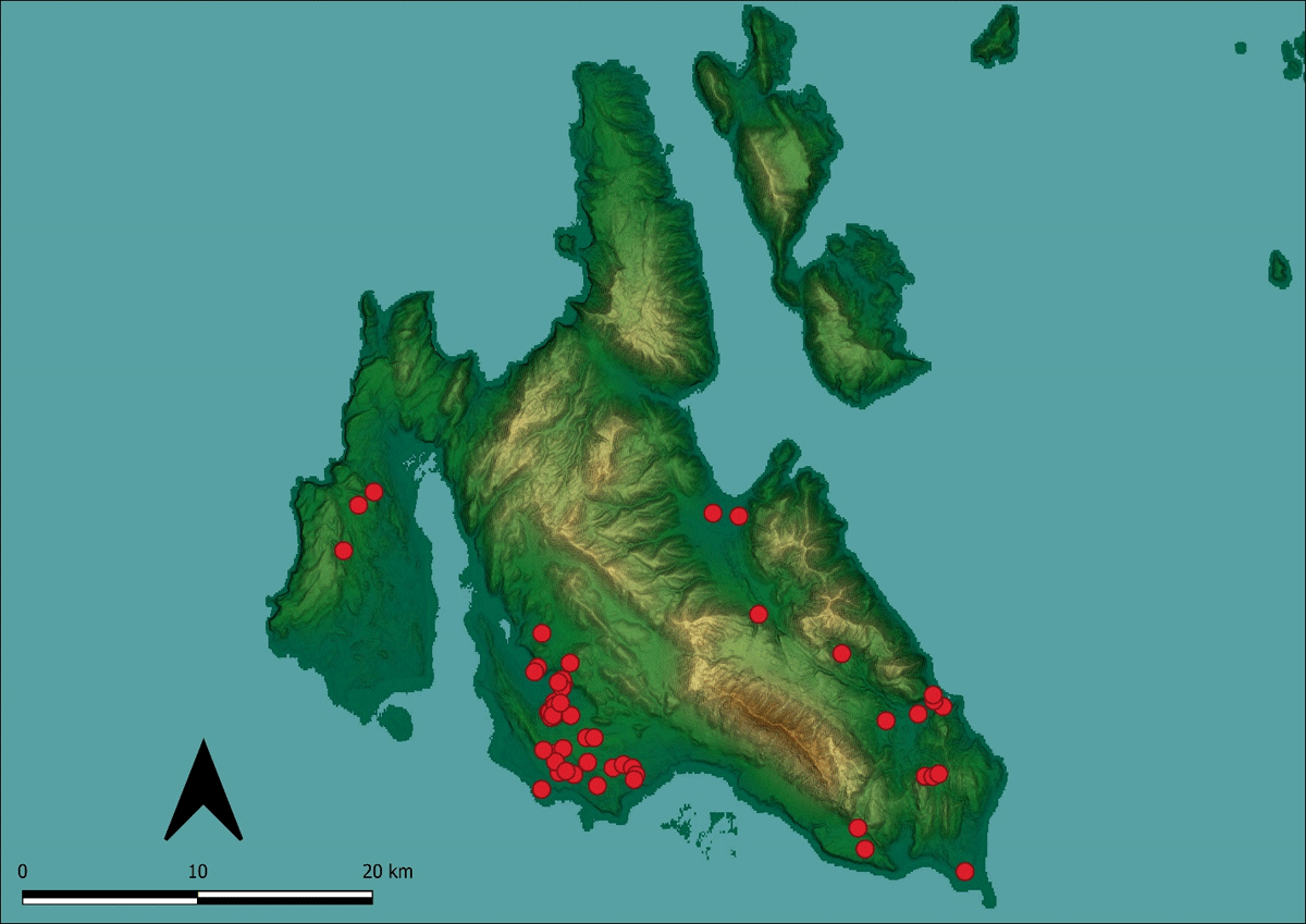
Figure 6
Kefalonia and the distribution of sites included in this study.
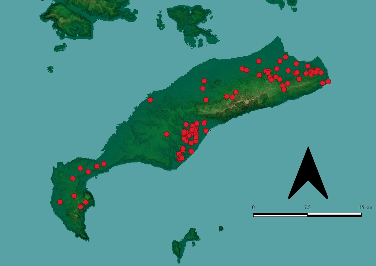
Figure 7
Kos and the distribution of sites included in this study.
Despite these provisos, the CPA yields discernible trends (Figure 8). Most strikingly, the Late and Final Neolithic eras display the shortest median time cost to the coastline in both Kea and Kefalonia, while the same is not true on Kos. On Kea, this correlates aptly with the maritime orientation of the Attic-Kephala culture prevalent during the Final Neolithic period, suggesting that coastal access figured prominently in the choice of settlement location (Broodbank 2000: 149), while the period appears to have been a time of maximum expansion in settlement (Davis 2001: 22), leading to the colonisation on several previously uninhabited islands of the Cyclades. Excavations at the Final Neolithic settlement at Kephala on Kea indicates a community predicated upon animal husbandry, farming, and fishing (Coleman 1977: 111), a pattern which may hold true for other contemporary settlements on Kea. For Kefalonia the Neolithic evidence is patchier, with only three sites known (Figure 9), though the median time cost is lower than for later periods on the same island. Increased exploration of Kefalonia’s landscape may help to clarify the nature of Neolithic settlement patterns. Kos, on the other hand, exhibits a higher median time cost to the coast than on both Kea and Kefalonia. This is remarkable, given that the Neolithic period is well represented on Kos (35 sites) and the fact that the island is comparable in size to Kea, yet considerably smaller than Kefalonia, which has a lower median coastal proximity. This suggests that there was a conscious choice to situate later Neolithic habitations at a greater time cost away from the coast than can be observed later on the same island, perhaps due to risks associated with living on the coast.
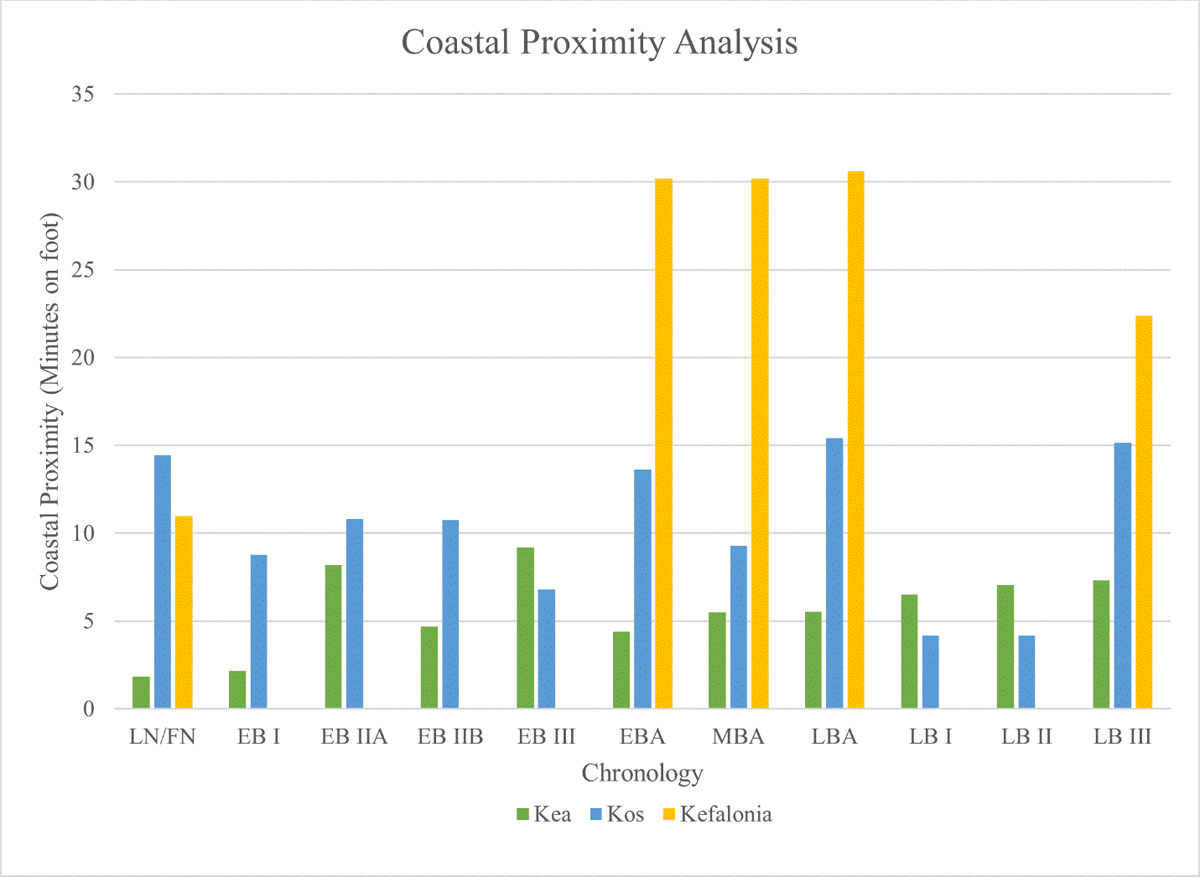
Figure 8
The tabulated data for the Coastal Proximity Analysis.
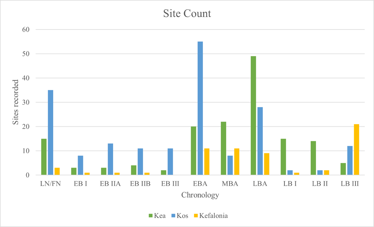
Figure 9
Number of sites for each period divided by island.
Addressing the discrete phases of the EBA poses a challenge due to the scant number of sites categorically aligned with each specific period, especially on Kefalonia, where EBA ceramics are poorly defined. Nonetheless, a slight increase in the median time cost is discernible on Kea, most notably in EB II early and EB III phases. For Kos there is a slight shift, with EB I and EB III having greater coastal proximity. EBA evidence on Kefalonia is notoriously difficult to place chronologically, due to the lack of clear EBA ceramic sequence (Souyoudzoglou-Haywood 1999: 46), though the CPV is close to ten times higher than that of Kea, indicating a lower incidence of habitation immediately on the coast. EB II early sees a subtle increase in the median time cost to the coast for Kos and a more substantial shift for Kea, during a time of ‘international’ exchange networks (Renfrew 1972). The continuity of activity at the notable coastal site of Ayia Irini until the close of EB II late injects a counterpoint to this general trend. However, this site may have been of sufficient size and power to mobilise enough warriors to defend itself (Broodbank 2000: 279–287), if EBA exchange networks carried the potential for violence. The considerably lower number of settlements of EB II late–III identified on Kea as opposed to Kos may indicate that the natural environment of Kos afforded greater protection against the so-called 4.2 ka climatic event (Bini et al. 2019: 555–577), which may have had a pronounced impact on the more arid Aegean islands such as Kea and could offer another explanation for the observed shift in coastal proximity.
The MBA witnesses a considerable resurgence in the number of sites on Kea and Kefalonia, although the granularity of the fieldwalking data precludes precise attribution to specific subphases within this period. The data manifests a slight increase in median time cost to the coast on Kea, while the reverse trend is observed on Kos, and the coastal site at Seraglio is likely to have been the island’s main settlement (Davis 1982: 39). This phase is also characterised by the re-establishment of activity at the principal site of Ayia Irini on Kea during the MBA (Gorogianni 2016: 138), as well as a contemporary demographic refilling of the coastal and near-coastal zones of northwest Kea. The settlement pattern of Kefalonia can be characterised by stability, with the EBA configuration of settlement patterns continuing into the MBA, without much change.
The LBA manifests a strikingly stable pattern of habitation on Kea, replete with a diversity of active sites throughout this period. Nevertheless, we confront another obstacle in the form of limited chronological resolution inherent in the ceramic data gathered from fieldwalking, which often bears imprecise temporal labels such as “Middle to Late Cycladic II” or simply “LBA”, owing to the challenges of dating weathered surface ceramics. A substantial corpus of sites falls under such fuzzy chronological labels. For Kea, many sites are identified in the earlier LBA phases, suggesting a sequential pattern of occupation with a propensity for short-term habitation before relocation. This stage resonates with broader transformations in the southern Aegean, marked by a move towards ‘farmhouse’ sites, a trend likewise observed in locales such as Crete, Thera, and Melos (Younger & Rehak 2008: 143; Davis 2008: 201), in addition to a general ‘colonisation of the interior’, with settlement expansion identifiable on the mainland in the Peloponnese and Attica (Rutter 1993: 781). It reflects an outward expansion from the principal MBA settlements into the rural landscape. This pattern may have been supported by the strength of the key trading node at Ayia Irini, part of a so-called ‘Western String’ trading route running from the metal sources at Lavrion in Attica, through selected key Cycladic ports, terminating in the Minoan palaces of Crete (Davis 1979; Schofield 1982; Berg 2006; Belza 2018). The prosperity generated by participation in such a network during the late MBA to early LBA (Jones 2021: 113) could have afforded an expansion into the countryside on Kea.
LB III unfolds differently across the three islands, each responding differently to considerable cultural shifts associated with the ‘Mycenaean’ presence in the Cyclades (Barber 1999) and wider Aegean (Dodecanese: Mee 1982; Crete: Wiener 2015) and Ionian islands (Souyoudzoglou-Haywood 1999: 136). On Kea, there is a stark contraction in site numbers, yet the coastal proximity of these LB III sites remains consistent. Perhaps interaction with the Palatial Greek mainland led to a consolidation of activity at fewer, central, perhaps more defensible, locations, though an additional factor is the disruption of exchange networks due to the Theran volcanic eruption (c. 1610 BCE). This may have led to a collapse in the settlement pattern that was previously supported by participation in the ‘Western String’ exchange network (Jones 2021: 113).
Kefalonia and Kos on the other hand experience an increase in LB III sites but display different spatial trends. Kos witnesses an increase in median time cost to the coast, while Kefalonia observes the reverse trend. Still, even the least proximal coastal sites on Kos remain a shorter travel time to the shore than those on Kefalonia. This surge in activity on Kefalonia is represented mostly by burial sites and could possibly be ascribed to an influx of people, likely from the Greek mainland (Souyoudzoglou-Haywood 1999: 136). This period witnesses the Mycenaean expansion into the Ionian islands, and the newly occupied sites, although at a shorter time cost to the coast than before, still maintain a greater inland bias compared to the patterns evident on smaller islands like Kea and Kos.
An additional outcome is an indication of how traditional Euclidean distance measurements and the CPA values compare. When looking at the ranking of the sites, there is an upward trend (Figure 10), suggesting that the CPV rank (e.g. 1 being the shortest) does correlate to Euclidean distance. There are, however a few notable exceptions, for example Site 24: ALA on Kefalonia which is 10th shortest travel time, though has the longest Euclidean distance towards the coast. In this case, the local topography is lower-lying without much elevation making the travel time much faster than sites which may have been closer in Euclidean terms, but had significant elevated obstacles en route, for example Koressia on Kea, which was ranked third closest in Euclidean distance, but 65th in the CPV. The latter can be explained by changes in palaeotopography, where reduced sea levels, as well as elevated topography created additional walking costs.
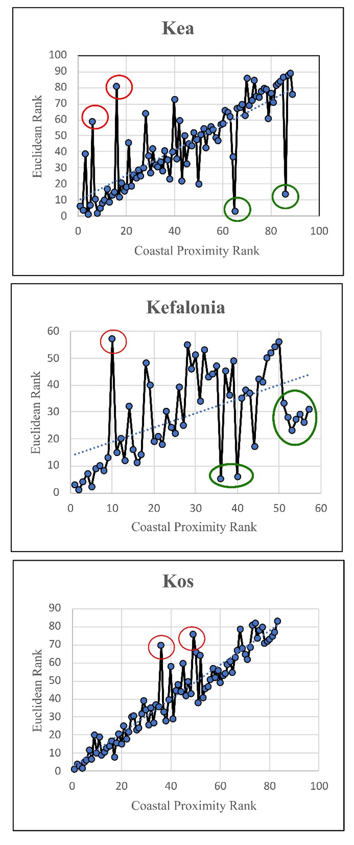
Figure 10
Plot of rankings of Costal Proximity values and Euclidean distance. Anomalies indicate divergences from the trend. Red indicates sites with a shorter travel time ranking than Euclidean Rank. Green indicates sites with a shorter Euclidean distance but higher travel time rank.
4. Conclusions
This short article has introduced the CPA concept, detailed its method, and applied it to three case studies focusing on prehistoric settlement patterns on island environments in Greece. The case studies highlight the differing use of islandscape on three Greek islands in prehistory and the changing circumstances of the social relationship between society and coastline (Figure 11).

Figure 11
‘Box and Whisker’ plots for the distribution of coastal proximity values on each island by period. The “X” refers to the mean value for coastal proximity, the boxes the lower and upper quartiles (interquartile range), while the “whiskers” represent a value 1.5 times the interquartile range. Data beyond these boundaries are outliers.
For Kea, its topography means that the coastline was only ever a relatively short distance away. Nevertheless, there is a much higher degree of coastscape engagement in specific periods. Settlement patterns are less clear in the EBA, but higher site numbers are registered during the MBA onwards towards LB II, after which site numbers decline. Kos on the other hand, sees a more consistent settlement pattern from FN to the end of the EBA, with a subsequent nucleation at a restricted number of sites from MBA to LB II, with a further increase in LB III. Median coastal proximity on Kos fluctuated from a low of 4 minutes in LB I, indicating a substantial nucleation particularly at the coastal Seraglio settlement, to a high of 15 minutes in LB III, indicating more activity slightly further inland. This process could have been influenced by Mycenaean contact, if not representing an actual movement of Mycenaeans to the island (Nuttall 2014).
For the larger Kefalonia island, coastscapes appear to have been less important to settlement patterns. The island has a considerably more elevated topography, with its peak sitting at 1628 m, compared to Kea’s 560 m and Kos’s 864 m. This results in greater slopes hindering movement from the interior to the coastline. As a result, CPV’s manifest as considerably higher than those observed on Kea and Kos. The coast appears to have been generally avoided on Kefalonia, with no major coastal settlements (Souyoudzoglou-Haywood 1999: 59), unlike those observed on Kea with FN Kephala and EBA-LBA Ayia Irini, and Kos with EBA-LBA Seraglio. The larger size of Kefalonia, and its elevated topography, may have afforded ancient people the opportunity to live further inland, though further work will be needed to determine whether there is some geomorphological process which may have obscured or destroyed potential coastal sites on the island.
The case studies highlight the need for finer resolution chronological data, though this issue notwithstanding, elucidate the spatial relationship between the different prehistoric peoples of these three islands, their coastlines, and how different social configurations used the same space in different ways. Such interpretations are possible with the holistic and humanistic perspective of CPA, incorporating spatiality, palaeotopography and human movement through the landscape.
Reproducibility
The data for this article can be found online here: https://doi.org/10.5281/zenodo.10634062.
Additional File
The additional file for this article can be found as follows:
Appendix 1
The following tables represent the sites included in the coastal proximity analysis, from the islands of Kea, Kos and Kefalonia. The spatial information for each site has been derived from maps provided in the relevant archaeological surveys. As a result, the spatial information is indicative, rather than definitive. DOI: https://doi.org/10.5334/jcaa.143.s1
Notes
[1] The following abbreviations are used in this paper: DEM: Digital Elevation Model; DBM: Digital Bathymetric Model; CPA: Coastal Proximity Analysis; CPV: Coastal Proximity value; QGIS: Quantum Geographic Information System; LCP: Least Cost Path; LN: Late Neolithic; FN: Final Neolithic; EBA: Early Bronze Age; MBA: Middle Bronze Age; LBA: Late Bronze Age.
[2] Regrettably, the Kefalonia Archaeology and History survey (Randsborg 2002) provides no maps or geospatial information associated with the 83 sites of prehistoric activity, making a CPA impossible.
Acknowledgements
I would like to express my thanks to Jenny Wallensten and the Swedish Institute at Athens for their support, as well as my colleagues at the National and Kapodistrian University of Athens. Michael Lindblom provided useful comments, Jovan Kovačević provided GIS assistance and my two peer-reviewers greatly enhanced this paper. Any deficiencies are my own.
Funding Information
Project: “Populating the coastal landscapes of Greece. Assessing coastal engagement in later prehistoric (7000 – 1100 BCE) southern Greece” funded by the Swedish Research Council’s (Vetenskapsrådet) International Postdoc in Humanities and Social Science, Project ID: 2022-06184.
Competing interests
The author has no competing interests to declare.