
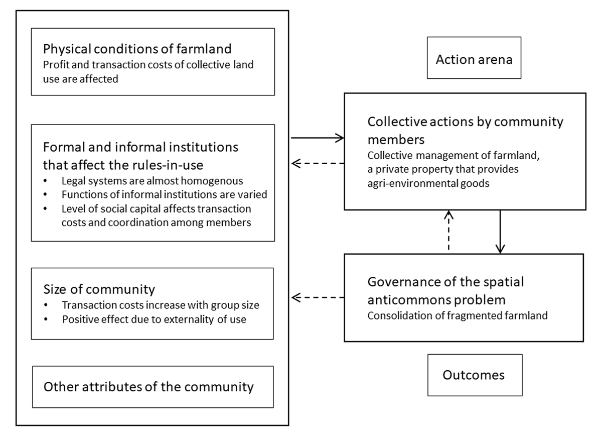
Figure 1
A framework to link factors and collective actions.
Note: The solid arrows represent the direct effects of factors, while the dashed arrows represent the feedback effects.
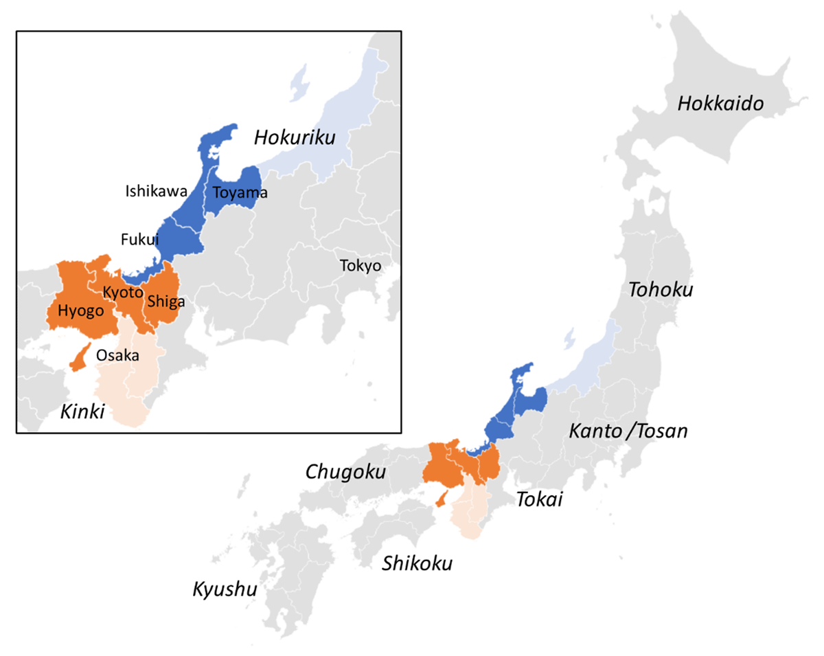
Figure 2
Location of study areas.
Note: The blue area represents the Hokuriku region, and the orange area represents the Kinki region. The dark-shaded area represents the study areas in the two regions. The areas in italics show the location of agricultural regions.
Table 1
Correspondence between the selected variables and theoretical conditions.
| VARIABLES | THEORETICAL GROUNDING | EXPECTED SIGN |
|---|---|---|
| Dependent variables | ||
| Existing community farming enterprises | Collective action level for farmland consolidation | |
| Rate of farmland concentration | ||
| Collective farm management | ||
| Independent variables | ||
| 1. Rate of farmland improvement | (1) Physical conditions of farmland that increase profit and decrease transaction costs of collective farmland use | + |
| 2. Community functions | (2) Levels of social capital that affect the transaction costs for collective actions and coordination among members | + |
| Activities for revitalizing communities | ||
| Number of local meetings | ||
| 3/4. Human and areal scale of the farmland market | (3) Size of the community, with negative effect by increasing transaction costs and positive effect by the externality of use | +/– Possibly inverse-U |
| Number of farmland-holding households | ||
| Ratio of farmland-holding households to total households | ||
| Paddy field area | ||
Table 2
Relationship between the rate of farmland improvement and farmland use by community farming enterprises.
| RATE OF FARMLAND IMPROVEMENT | 0 | 0–0.2 | 0.2–0.4 | 0.4–0.6 | 0.6–0.8 | 0.8–1.0 | 1 | AVERAGE |
|---|---|---|---|---|---|---|---|---|
| Number of rural communities | 6,106 | 966 | 413 | 452 | 773 | 1,364 | 1,954 | 12,028 |
| (Percentage) | (50.8) | (8.0) | (3.4) | (3.8) | (6.4) | (11.3) | (16.2) | (100.0) |
| Existing community farming enterprises | 19.9 | 34.9 | 40.2 | 38.5 | 45.3 | 52.1 | 50.2 | 32.7 |
| Farmland concentration rate | 8.5 | 17.2 | 19.8 | 19.0 | 25.4 | 29.0 | 26.6 | 16.3 |
| Collective farm management and operation by community farming enterprises | 4.9 | 11.4 | 16.9 | 14.2 | 18.8 | 22.9 | 21.3 | 11.8 |
[i] Source: Survey of Community Farming, Database of Regional Agriculture, Census of Agriculture and Forestry.
Note: “Number of rural communities” and the percentage indicate the number of classified communities and the percentage of the total number of rural communities, respectively. “Existing community farming enterprises” indicate the percentage of the number of corresponding rural communities to the total number of the classification. For example, 6,106 communities (50.8% of the total) have no farmland improvement, and community farming enterprises exist in 19.9% of the communities with a zero farmland improvement rate.
Table 3
Relationship between the number of meetings and farmland use for community farming.
| NUMBER OF LOCAL MEETINGS | 0 | 1–2 | 3–6 | 7–12 | 13–18 | 19+ | AVERAGE |
|---|---|---|---|---|---|---|---|
| Number of rural communities | 211 | 605 | 2,408 | 3,413 | 2,205 | 3,186 | 12,028 |
| (Percentage) | (1.8) | (5.0) | (20.0) | (28.4) | (18.3) | (26.5) | (100.0) |
| Existing community farming enterprises | 4.3 | 11.4 | 20.1 | 31.5 | 35.2 | 47.8 | 32.7 |
| Farmland concentration rate | 2.0 | 5.8 | 10.1 | 15.9 | 17.7 | 23.6 | 16.3 |
| Collective farm management and operation by community farming enterprises | 2.4 | 3.5 | 6.6 | 11.7 | 11.8 | 18.0 | 11.8 |
[i] Source: Survey of Community Farming, Database of Regional Agriculture, Census of Agriculture and Forestry.
Note: See the notes for Table 2.
Table 4
Quantitative analysis of farmland use by community farming enterprises.
| EXISTING COMMUNITY FARMING ENTERPRISES | RATE OF FARMLAND CONCENTRATION | COLLECTIVE FARM MANAGEMENT AND OPERATION BY COMMUNITY FARMS | ||||
|---|---|---|---|---|---|---|
| COEF. | T | COEF. | T | COEF. | T | |
| 1. Farmland improvement rate | 0.0886 | 4.99 *** | 0.0646 | 5.57 *** | 0.0616 | 4.79 *** |
| 2. Community functions | ||||||
| Community- revitalizing activities | 0.0133 | 4.20 *** | 0.0080 | 3.80 *** | 0.0005 | 0.22 |
| Number of local meetings | 0.0025 | 5.36 *** | 0.0016 | 5.88 *** | 0.0017 | 4.64 *** |
| 3. Human scale of the farmland market | ||||||
| Number of farmland-holding households | 0.0025 | 4.19 *** | 0.0008 | 2.08 ** | 0.0009 | 2.09 ** |
| Squared number of farmland-holding households | –1.5.E–05 | 3.54 *** | –6.5.E–06 | –2.42 ** | –8.4.E–06 | 2.84 *** |
| Percentage of farmland-holding households | 0.0915 | 4.66 *** | 0.0466 | 3.69 *** | 0.0090 | 0.65 |
| 4. Areal scale of farmland market | ||||||
| Paddy field area | 0.0079 | 9.68 *** | 0.0034 | 6.96 *** | 0.0032 | 5.88 *** |
| Squared paddy field area | –4.4.E–05 | –7.77 *** | –2.2.E–05 | –6.67 *** | –1.5.E–05 | –4.25 *** |
| 5. Geographic conditions | ||||||
| Ratio of urbanization promotion area | 0.0623 | 1.90 * | 0.0297 | –1.52 | –0.0263 | –1.19 |
| Ratio of agricultural promotion area | 0.0355 | 1.24 | 0.0179 | 0.96 | 0.0049 | 0.22 |
| Ratio of farmland area to total land area | 0.0377 | 1.04 | 0.0543 | 2.23 ** | 0.0431 | 1.45 |
| Ratio of paddy fields to total farmland | 0.0244 | 0.85 | 0.0383 | 2.10 ** | 0.0015 | 0.08 |
| Within 30 minutes of DID | 0.0014 | 0.09 | 0.0067 | 0.67 | 0.0011 | 0.11 |
| 6. Population conditions | ||||||
| Percentage of population aged 65 and over | 0.0260 | 0.64 | 0.0290 | –1.10 | 0.0216 | 0.76 |
| Ratio of population employed in agriculture and forestry | 0.0118 | 0.29 | 0.0534 | –2.06 *** | 0.0484 | –1.81 * |
| Value at the top of the inverted U-shape | ||||||
| Number of farmland-holding households | 84.9 | 62.5 | 52.1 | |||
| Paddy field area | 90.2 | 79.1 | 105.1 | |||
| No. of observations | 12,028 | |||||
| Degree of freedom | 10,648 | |||||
| R-squared | 0.492 | 0.444 | 0.458 | |||
| F-statistics for overall significance (p-value) | 47.43 (0.00) | 27.73 (0.00) | 11.60 (0.00) | |||
[i] 1. ***, **, and * are significantly different from zero at the 1%, 5%, and 10% levels, respectively.
2. We use standard errors that are robust to the heteroskedasticity and the cluster structure for each former municipality.
3. The value at the top of the inverted U-shape is calculated when the variable and its squared term are significantly different from zero at the 5% level.
4. The notation “–1.5.E-05” in the table represents –1.5 × 0.1 to the fifth power.
5. DID = densely inhabited district.