
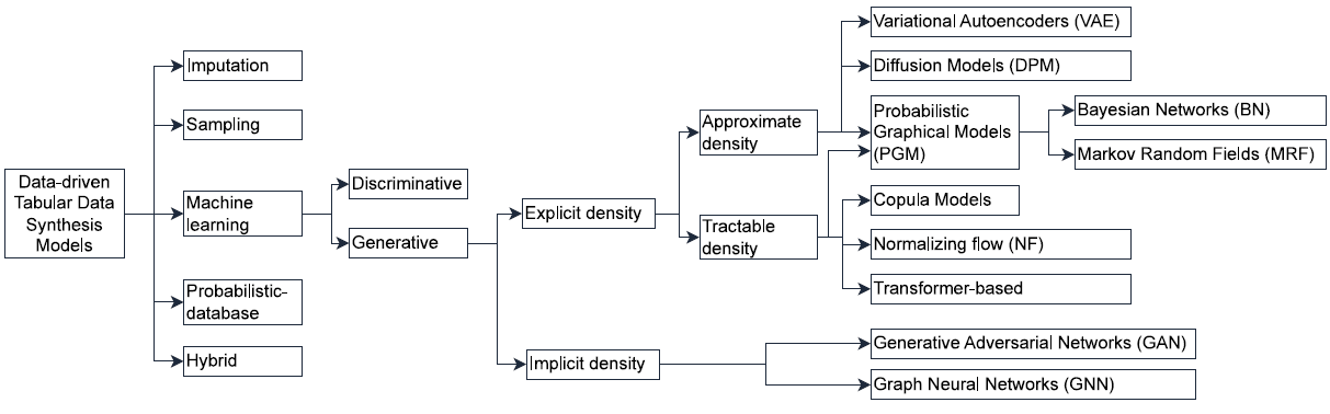
Figure 1
Taxonomy of TDS models (illustration taken from Davila et al. (2025, Fig. 1)).
Table 1
13 tools chosen for the benchmark.
| MODEL | TDS TOOL |
|---|---|
| Sampling | SMOTE (Cantalupo, 2021; Lemaître, Nogueira, and Aridas, 2017) |
| Bayesian Networks | PrivBayes (Zhang et al., 2017) |
| GAN | CTGAN (Xu et al., 2019), CTAB-GAN+ (Zhao et al., 2021), GANBLR++ (Zhang et al., 2022) |
| VAE | TVAE (Xu et al., 2019) |
| Diffusion (DPM) | TabDDPM (Kotelnikov et al., 2023) |
| Graph NN | GOGGLE (Liu et al., 2023) |
| Transformer | GReaT (Borisov et al., 2023), REalTabFormer (Solatorio and Dupriez, 2023), TabuLa (Zhao, Birke, and Chen, 2025) |
| Hybrid | AutoDiff (Suh et al., 2023), TabSyn (Zhang et al., 2024) |
Table 2
| DATASET | COLUMN NUMBER | ROW NUMBER | CATEGORICAL COLUMNS | CONTINUOUS COLUMNS | MIXED COLUMNS | ML TASK |
|---|---|---|---|---|---|---|
| abalone (Nash et al., 1994) | 8 | 4177 | 1 | 7 | 0 | Regression |
| adult (Becker and Kohavi, 1996) | 14 | 48842 | 9 | 3 | 2 | Classification |
| airline (Banerjee, 2016) | 10 | 50000 | 8 | 2 | 0 | Regression |
| california (Nugent, n.d.) | 5 | 20433 | 1 | 4 | 0 | Regression |
| cardio (Janosi et al., 1989) | 12 | 70000 | 7 | 5 | 0 | Classification |
| churn2 (BlastChar, 2017) | 12 | 10000 | 5 | 6 | 1 | Classification |
| diabetes (Kahn, n.d.) | 9 | 768 | 2 | 7 | 0 | Classification |
| higgs-small (Whiteson, 2014) | 29 | 62751 | 1 | 28 | 0 | Classification |
| house (Torgo, 2014) | 16 | 22784 | 0 | 16 | 0 | Regression |
| insurance (Kumar, 2020) | 6 | 1338 | 3 | 3 | 0 | Regression |
| king (harlfoxem, 2016) | 19 | 21613 | 7 | 10 | 2 | Regression |
| loan (Quinlan, 1987) | 12 | 5000 | 6 | 6 | 0 | Classification |
| miniboone-small (Roe, 2005) | 51 | 50000 | 1 | 50 | 0 | Classification |
| payroll-small (City of Los Angeles, 2013) | 12 | 50000 | 4 | 8 | 0 | Regression |
| wilt (Johnson, 2013) | 6 | 4339 | 1 | 5 | 0 | Classification |
Table 3
| EVALUATION | CHALLENGE | EVALUATION FOCUS | METRICS |
|---|---|---|---|
| Dataset Imbalance | Ensuring that the tool is able to capture the real column distributions, even though there are imbalances in the classes | Class distribution alignment | Continuous: Wasserstein Distance, KS Statistic, Correlation Differences. Categorical: Jensen–Shannon Divergence, KL Divergence, Percentage Class Count Difference |
| Data Augmentation | Guaranteeing that the synthetic data generated remains realistic and meaningful | Similarity and meaningful variability of new data points | Continuous: Wasserstein Distance, KS Statistic, Correlation Differences, Quantile Comparison. Categorical: Jensen–Shannon Divergence, Percentage Number of Classes Difference |
| Missing Values | Making certain the tools are able to capture the key characteristics of the real dataset, even if it includes different levels of missing values | Similarity to original distributions | Continuous: Wasserstein Distance, Quantile Comparison. Categorical: Jensen-Shannon Divergence, Percentage Class Count Difference, Percentage Number of Classes Difference |
| Privacy | Ensuring whether the tools can generate truly synthetic data points rather than replicating the original data, which could potentially expose sensitive information | Resemblance of synthetic records and real data and anonymity levels | Distance to Closest Record (DCR), Nearest Neighbor Distance Ratio (NNDR) |
| Machine Learning Utility | Enabling effective ML training with synthetic data | Synthetic datasets used to train ML models for classification and regression tasks | Accuracy, Area Under the Receiver Operating Characteristic Curve (AUC), F1 Score (micro, macro, weighted), Explained Variance Score, Mean Absolute Error (MAE), and R2 Score. |
| Performance | Ensuring synthetic data is generated within reasonable time frames while minimizing computational resource usage and maintaining scalability | Measure the computational resource usage and time required for data generation | CPU Usage, GPU Usage, Memory Usage, Total Runtime |
Table 4
Normalization of datasets in the original experiments of different TDS tools.
| TOOL | NORMALIZATION STRATEGY |
|---|---|
| PrivBayes | Only discrete columns, no normalization |
| CTGAN / TVAE | Mode-specific normalization applied to all X |
| GANBLR++ | Ordinal encoding for all columns; numerical treated as discrete |
| TabDDPM | Normalization of complete X (per code in data.py) |
| GOGGLE | No normalization (raw tensors from get_dataloader) |
| GReaT | No normalization; textual encoding of all columns |
| REaLTabFormer | Numerical columns normalized into fixed-length, digit-aligned string tokens |
| TabuLa | No normalization; continuous values directly as text tokens |
| AutoDiff | All numerical X normalized (Stasy: min–max; Tab: Gaussian quantile). |
| TabSyn | Z-score normalization of all numerical X |
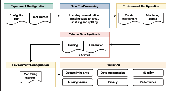
Figure 2
Overview of the benchmark architecture, which automates configuration and analysis, ensuring reproducibility and consistency across tools and datasets.
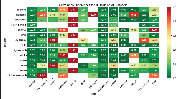
Figure 3
Heatmap showing the correlation difference for various TDS tools and use cases, where zero indicates perfect preservation of inter-column correlations, and one represents the maximum difference. Empty cells denote cases where no dataset was generated due to intentional resource constraints.
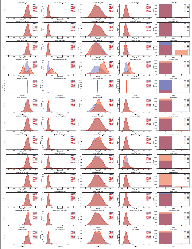
Figure 4
Distribution comparison for Wilt, with one row per TDS tool. For continuous columns, real data is in blue and synthetic in red. For categorical columns, bars show class counts with real data in blue and synthetic in red. The five synthetic distributions occasionally overlap completely. GOGGLE collapsed and therefore shows exploding densities.
Table 5
Dataset imbalance evaluation for all tools, averaged across datasets and normalized using Min–Max scaling, highlighting the top-performing tools (SMOTE, REalTabFormer, and TabSyn).
| TOOL | WASSERSTEIN DISTANCE | KS STATISTIC | CORRELATION DIFFERENCE | JS DIVERGENCE | KL DIVERGENCE | PERCENTAGE COUNT DIFFERENCE |
|---|---|---|---|---|---|---|
| AutoDiff | 0.218 | 0.164 | 0.146 | 0.211 | 0.134 | 0.154 |
| CTAB-GAN+ | 0.324 | 0.416 | 0.265 | 0.344 | 0.335 | 0.117 |
| CTGAN | 0.286 | 0.482 | 0.308 | 0.382 | 0.411 | 0.528 |
| GANBLR++ | 0.692 | 0.748 | 0.542 | 0.714 | 0.659 | 0.489 |
| GReaT | 0.576 | 0.674 | 0.209 | 0.653 | 0.189 | 0.246 |
| REalTabFormer | 0.113 | 0.294 | 0.041 | 0.185 | 0.138 | 0.002 |
| SMOTE | 0.063 | 0.062 | 0.176 | 0.015 | 0.019 | 0.198 |
| TabDDPM | 0.344 | 0.325 | 0.053 | 0.294 | 0.276 | 0.861 |
| TabSyn | 0.040 | 0.128 | 0.324 | 0.094 | 0.109 | 0.176 |
| TabuLaMiddle | 0.513 | 0.641 | 0.183 | 0.588 | 0.201 | 0.233 |
| TVAE | 0.317 | 0.543 | 0.327 | 0.423 | 0.346 | 0.414 |
Table 6
Augmentation evaluation results for all tools averaged across datasets and normalized using Min–Max scaling. The top-performing tools: TabSyn, SMOTE, REalTabFormer, and TabDDPM.
| TOOL | WASSERSTEIN DISTANCE | KS STATISTIC | CORRELATION DIFFERENCE | QUANTILE COMPARISON | JS DIVERGENCE | PERCENTAGE NUMBER CLASSES DIFFERENCE |
|---|---|---|---|---|---|---|
| AutoDiff | 0.218 | 0.164 | 0.146 | 0.197 | 0.211 | 0.028 |
| CTAB-GAN+ | 0.324 | 0.416 | 0.265 | 0.287 | 0.344 | 0.045 |
| CTGAN | 0.286 | 0.416 | 0.265 | 0.226 | 0.382 | 0.014 |
| GANBLR++ | 0.692 | 0.748 | 0.542 | 0.670 | 0.714 | 0.096 |
| GReaT | 0.576 | 0.674 | 0.209 | 0.543 | 0.653 | 0.245 |
| REalTabFormer | 0.113 | 0.294 | 0.041 | 0.092 | 0.185 | 0.021 |
| SMOTE | 0.063 | 0.062 | 0.176 | 0.071 | 0.015 | 0.126 |
| TabDDPM | 0.344 | 0.325 | 0.053 | 0.259 | 0.294 | 0.006 |
| TabSyn | 0.040 | 0.128 | 0.324 | 0.066 | 0.094 | 0.123 |
| TabuLaMiddle | 0.513 | 0.641 | 0.183 | 0.465 | 0.588 | 0.332 |
| TVAE | 0.317 | 0.543 | 0.327 | 0.287 | 0.423 | 0.069 |
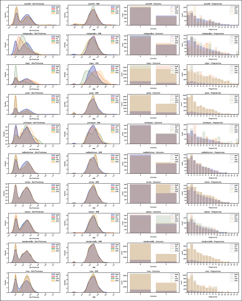
Figure 5
Distribution comparison for the Diabetes dataset, with 5%, 10% and 20% missing values. The real data distribution is plotted in blue, and synthetic data in red, green and orange. Continuous columns as density plots and categorical columns as bar plots.
Table 7
Missing-values evaluation results normalized using Min–Max scaling.
| TOOL | WASSERSTEIN DISTANCE | KS STATISTIC | CORRELATION DIFFERENCE | QUANTILE COMPARISON | JS DIVERGENCE | KL DIVERGENCE | PERCENTAGE COUNT DIFFERENCE | PERCENTAGE NUM CLASSES DIFFERENCE |
|---|---|---|---|---|---|---|---|---|
| (a) 5% Missing Values | ||||||||
| AutoDiff | 0.249 | 0.178 | 0.621 | 0.194 | 0.399 | 0.051 | 0.089 | 0.000 |
| CTAB-GAN+ | 0.412 | 0.412 | 0.217 | 0.408 | 0.420 | 0.545 | 0.019 | 0.093 |
| CTGAN | 0.829 | 0.930 | 0.669 | 0.855 | 0.846 | 0.879 | 0.722 | 0.061 |
| GReaT | 0.744 | 0.681 | 0.578 | 0.731 | 0.843 | 0.091 | 0.498 | 0.138 |
| REalTabFormer | 0.251 | 0.402 | 0.121 | 0.278 | 0.460 | 0.560 | 0.004 | 0.147 |
| SMOTE | 0.061 | 0.072 | 0.182 | 0.062 | 0.048 | 0.051 | 0.376 | 0.000 |
| TabSyn | 0.074 | 0.112 | 0.418 | 0.052 | 0.123 | 0.030 | 0.045 | 1.000 |
| TabuLaMiddle | 0.362 | 0.438 | 0.091 | 0.401 | 0.531 | 0.018 | 0.452 | 0.055 |
| TVAE | 0.830 | 0.879 | 0.378 | 0.835 | 0.842 | 0.422 | 0.478 | 0.186 |
| (b) 10% Missing Values | ||||||||
| AutoDiff | 0.368 | 0.182 | 0.642 | 0.319 | 0.415 | 0.074 | 0.069 | 0.000 |
| CTAB-GAN+ | 0.798 | 0.605 | 0.471 | 0.799 | 0.635 | 0.669 | 0.147 | 0.092 |
| CTGAN | 0.725 | 0.963 | 0.523 | 0.753 | 0.872 | 0.875 | 0.734 | 0.034 |
| GReaT | 0.753 | 0.711 | 0.583 | 0.735 | 0.887 | 0.077 | 0.495 | 0.167 |
| REalTabFormer | 0.269 | 0.436 | 0.108 | 0.263 | 0.469 | 0.531 | 0.004 | 0.165 |
| SMOTE | 0.067 | 0.065 | 0.181 | 0.029 | 0.043 | 0.047 | 0.368 | 0.000 |
| TabSyn | 0.072 | 0.092 | 0.000 | 0.038 | 0.067 | 0.075 | 0.042 | 0.000 |
| TabuLaMiddle | 0.348 | 0.398 | 0.098 | 0.382 | 0.384 | 0.015 | 0.437 | 0.097 |
| TVAE | 0.735 | 0.984 | 0.537 | 0.789 | 0.804 | 0.399 | 0.459 | 0.261 |
| (c) 20% Missing Values | ||||||||
| AutoDiff | 0.405 | 0.184 | 0.589 | 0.385 | 0.386 | 0.058 | 0.081 | 0.000 |
| CTAB-GAN+ | 0.378 | 0.442 | 0.288 | 0.419 | 0.420 | 0.356 | 0.031 | 0.092 |
| CTGAN | 0.911 | 1.000 | 0.662 | 0.976 | 0.925 | 0.904 | 0.732 | 0.042 |
| GReaT | 0.769 | 0.678 | 0.563 | 0.782 | 0.863 | 0.071 | 0.501 | 0.129 |
| REalTabFormer | 0.267 | 0.435 | 0.128 | 0.336 | 0.492 | 0.433 | 0.005 | 0.138 |
| SMOTE | 0.049 | 0.082 | 0.162 | 0.071 | 0.051 | 0.049 | 0.378 | 0.000 |
| TabSyn | 0.502 | 0.972 | 0.231 | 0.533 | 0.835 | 0.061 | 0.021 | 0.033 |
| TabuLaMiddle | 0.334 | 0.411 | 0.116 | 0.406 | 0.466 | 0.520 | 0.451 | 0.057 |
| TVAE | 0.647 | 0.893 | 0.303 | 0.658 | 0.750 | 0.311 | 0.479 | 0.148 |
Table 8
Privacy results for all tools averaged across datasets and normalized using Min-Max scaling, highlighting the top-performing tools (CTAB-GAN+, REalTabFormer, and TabDDPM). The best score is one, and the worst is zero.
| TOOL | DISTANCE TO CLOSEST RECORD | NEAREST NEIGHBOR DISTANCE RATIO |
|---|---|---|
| AutoDiff | 0.162 | 0.847 |
| CTAB-GAN+ | 0.139 | 0.870 |
| CTGAN | 0.230 | 0.844 |
| GReaT | 0.046 | 0.751 |
| REalTabFormer | 0.283 | 0.781 |
| SMOTE | 0.032 | 0.342 |
| TabSyn | 0.261 | 0.750 |
| TabDDPM | 0.329 | 0.810 |
| TabuLaMiddle | 0.062 | 0.438 |
| TVAE | 0.101 | 0.837 |
Table 9
Classifiers and regressors used for the ML utility evaluation.
| CLASSIFICATION METHODS | REGRESSION METHODS |
|---|---|
| Decision Trees | Bayesian Ridge Regression |
| Gaussian Naive Bayes (NB) | Lasso Regression |
| K-Nearest Neighbors (KNN) | Linear Regression |
| Linear Support Vector Machine (SVM) | Ridge Regression |
| Logistic Regression | |
| Multilayer Perceptron (MLP) | |
| Perceptron | |
| Random Forest | |
| Radial Support Vector Machine (SVM) |
Table 10
ML utility results showing the difference between the model’s performance trained with real datasets and trained with synthetic datasets. For all metrics, if the difference is negative, the model performed better with synthetic data than with real data. If the difference is positive, the model performed worse.
| TOOL | ACCURACY | AUC | F1 MICRO | F1 MACRO | F1 WEIGHTED | EVS | INVERSE MAE | R2 SCORE |
|---|---|---|---|---|---|---|---|---|
| AutoDiff | –0.072 | 0.010 | –0.070 | –0.009 | –0.080 | 0.038 | 0.009 | 0.062 |
| CTAB-GAN+ | –0.052 | 0.074 | –0.046 | 0.071 | 0.053 | 0.176 | 0.145 | 0.172 |
| CTGAN | 0.089 | 0.046 | 0.081 | 0.053 | 0.093 | 0.193 | 0.472 | 0.192 |
| GANBLR++ | 0.118 | 0.152 | 0.121 | 0.156 | 0.137 | 0.548 | 0.342 | 0.546 |
| GReaT | 0.043 | 0.051 | 0.040 | 0.070 | 0.033 | 0.395 | 0.398 | 0.665 |
| REalTabFormer | –0.024 | –0.029 | –0.020 | –0.028 | –0.023 | 0.003 | –0.026 | 0.003 |
| SMOTE | –0.011 | –0.014 | –0.013 | –0.017 | –0.016 | 0.143 | 0.028 | 0.145 |
| TabDDPM | 0.019 | –0.031 | 0.017 | –0.023 | 0.010 | 0.034 | 0.182 | 0.035 |
| TabSyn | –0.046 | –0.041 | –0.043 | –0.040 | –0.078 | 0.018 | –0.035 | 0.017 |
| TabuLaMiddle | –0.063 | –0.072 | –0.059 | –0.052 | –0.080 | 0.204 | 0.066 | 0.011 |
| TVAE | –0.024 | –0.015 | –0.021 | –0.006 | –0.025 | 0.210 | 0.159 | 0.346 |
Table 11
Performance results for all tools averaged across datasets. Top-performing tools are SMOTE and PrivBayes; REalTabFormer shows the longest runtime and high resource usage.
| TOOL | MEAN CPU (%) | MAX CPU (%) | MEAN MEMORY (%) | MAX MEMORY (%) | MEAN GPU (%) | MAX GPU (%) | RUNTIME (S) |
|---|---|---|---|---|---|---|---|
| AutoDiff | 14 | 24 | 15 | 16 | 7 | 37 | 3240 |
| CTAB-GAN+ | 18 | 28 | 7 | 8 | 34 | 56 | 863 |
| CTGAN | 13 | 59 | 13 | 25 | 32 | 36 | 572 |
| GANBLR++ | 27 | 88 | 16 | 19 | 0 | 0 | 1790 |
| GOGGLE | 45 | 56 | 23 | 24 | 0 | 0 | 1106 |
| GReaT | 9 | 22 | 13 | 14 | 77 | 86 | 3714 |
| PrivBayes | 17 | 32 | 18 | 19 | 0 | 0 | 106 |
| REalTabFormer | 10 | 37 | 21 | 39 | 28 | 77 | 7682 |
| SMOTE | 25 | 38 | 17 | 17 | 0 | 0 | 248 |
| TabDDPM | 11 | 36 | 19 | 20 | 20 | 31 | 666 |
| TabSyn | 17 | 25 | 19 | 22 | 13 | 57 | 317 |
| TabuLaMiddle | 25 | 33 | 23 | 23 | 76 | 90 | 1097 |
| TVAE | 12 | 90 | 17 | 22 | 13 | 15 | 465 |

Figure 6
Spider web diagram summarizing model performance across the six benchmark dimensions. The scores are calculated by aggregating each dimension and are scaled 1–10.
Table 12
TDS tools and required packages.
| TDS TOOL | PACKAGE REQUIREMENTS |
|---|---|
| SMOTE | pandas==2.2.2, numpy==2.0.0, scikit-learn==1.5.2, imbalanced-learn==0.13.0 |
| PrivBayes | diffprivlib==0.6.3, dill==0.3.7, dython==0.6.8, joblib==1.2.0, lifelines==0.27.8, matplotlib==3.7.2, numpy==1.26.0, pandas==1.3.4, pyjanitor==0.26.0, pandas_flavor==0.6.0, scikit_learn==1.3.0, scipy==1.11.3, seaborn==0.13.0, thomas_core==0.1.3, synthetic-data-generation, torch, gpustat |
| CTGAN | tqdm==4.66.5, torch==2.1.0, numpy==2.0.0, pandas==2.2.2, scikit-learn==1.5.2, ctgan, joblib==1.4.2, rdt==1.7.0 |
| CTAB-GAN+ | numpy==1.21.0, torch==1.10.0+cu113, torchvision==0.11.1+cu113, torchaudio==0.10.0+cu113, pandas==1.2.1, scikit-learn==0.24.1, dython==0.6.4.post1, scipy, gpustat, tqdm, -f https://download.pytorch.org/whl/torch_stable.html |
| GANBLR++ | ganblr |
| TVAE | tqdm==4.66.5, torch==2.1.0, numpy==2.0.0, pandas==2.2.2, scikit-learn==1.5.2, ctgan, joblib==1.4.2, rdt==1.7.0 |
| TabDDPM | catboost==1.0.3, category-encoders==2.3.0, dython==0.5.1, icecream==2.1.2, libzero==0.0.8, numpy==1.21.4, optuna==2.10.1, pandas==1.3.4, pyarrow==6.0.0, rtdl==0.0.9, scikit-learn==1.0.2, scipy==1.7.2, skorch==0.11.0, tomli-w==0.4.0, tomli==1.2.2, tqdm==4.62.3 |
| GOGGLE | chardet==5.1.0, cvxpy==1.1, dgl==0.9.0, geomloss==0.2.5, matplotlib==3.7.0, numpy==1.23.0, packaging==21.3, pandas==1.4.3, pgmpy==0.1.21, scikit-learn==1.1.1, seaborn==0.12.2, synthcity==0.2.2, torch==1.12.0, torch-geometric==2.2.0, torch-sparse==0.6.16, torch_scatter==2.1.0 |
| GReaT | datasets≥2.5.2, numpy≥1.23.1, pandas≥1.4.4, scikit_learn≥1.1.1, torch≥1.10.2, tqdm≥4.64.1, transformers≥4.22.1, accelerate≥0.20.1 |
| REalTabFormer | torch, bandit≥1.6.2,<2.0, black~=22.0, build~=0.9.0, import-linter[toml]==1.2.6, openpyxl~=3.0.10, pre-commit≥2.9.2,<3.0, pylint≥2.5.2,<3.0, pytest-cov~=3.0, pytest-mock≥1.7.1,<2.0, pytest-xdist[psutil]~=2.2.1, pytest~=6.2, trufflehog~=2.1, twine~=4.0.1, pandas, datasets, scikit-learn, transformers, realtabformer |
| TabuLa | datasets≥2.5.2, numpy≥1.24.2, pandas≥1.4.4, scikit_learn≥1.1.1, torch≥1.10.2, tqdm≥4.64.1, transformers≥4.22.1 |
| AutoDiff | numpy==2.0.0, pandas==2.2.2, scikit-learn==1.5.2, scipy==1.10.1, torch==2.1.0, gpustat==1.0.0, psutil==5.9.4, tqdm==4.65.0, ipywidgets==7.8.5, jupyter==1.0.0, matplotlib==3.7.1 |
| TabSyn | numpy==2.0.0, pandas==2.2.2, scikit-learn==1.5.2, scipy==1.10.1, torch==2.1.0, icecream==2.1.2, category_encoders==2.3.0, imbalanced-learn==0.14.0, transformers==4.25.0, datasets==2.8.0, openpyxl==3.1.2, xgboost==1.7.5 |