
1 Introduction
Data is essential in many domains; however, it is often unavailable or restricted due to privacy concerns (European Parliament, 2023). Synthetic data is a possible solution, providing datasets that mimic real data while improving scalability, privacy, and new scenario simulations (Xu et al., 2019). This study focuses on tabular data synthesis (TDS), where models replicate real dataset characteristics such as column count, data types, distributions, correlations, and integrity constraints. Unlike other tabular generation methods that rely on schema or rule-based statistics (e.g., Bruno and Chaudhuri, 2005; Gray et al., 1994; Neufeld, Moerkotte, and Lockemann, 1993), TDS directly models real data properties.
Previous work introduced a taxonomy for TDS models (Figure 1; Davila et al., 2025) identified key use cases and challenges, such as handling class imbalance, missing values, and generating realistic samples without replicating input data when (i) augmenting datasets, (ii) ensuring privacy, or (iii) creating scenario-specific data. However, the assessment was limited to the reported results of each tool.
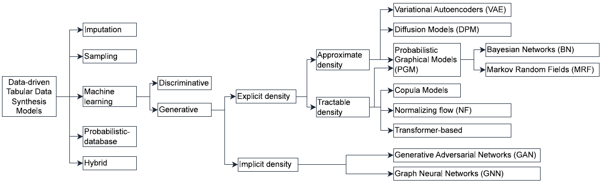
Figure 1
Taxonomy of TDS models (illustration taken from Davila et al. (2025, Fig. 1)).
Several benchmarks have been proposed to systematically evaluate TDS models across diverse domains. SynthRO (Santangelo and Others, 2025) is a dashboard-based framework used for health-related synthetic tabular data, assessing resemblance, utility, and privacy metrics with a focus on electronic health records. A prominent benchmark, Synthcity (Qian, Davis, and van der Schaar, 2023), offers a comprehensive Python library that evaluates fidelity, utility, fairness, and privacy across various data modalities and use cases. The SDGym benchmark, part of SDV (Patki, Wedge, and Veeramachaneni, 2016), compares some of the main TDS models based on correlation, data proximity, and computational efficiency.
Our benchmark builds on these previous works to create a comprehensive evaluation across six critical dimensions in TDS: handling dataset imbalance, data augmentation, managing missing values, ensuring privacy, assessing ML utility, and computational performance. The 15 datasets used cover the use cases of these dimensions. We present a comprehensive experiment with 13 state-of-the-art TDS tools, evaluating a wide range of models, including Sampling, Bayesian Networks (BN), Generative Adversarial Networks (GAN), Variational Autoencoders (VAE), Diffusion, Graph Neural Networks (GNN), Transformers, and Hybrid models, as shown in Figure 1.
Importantly, we focus on end-user scenarios, evaluating tools on prosumer hardware, where high-performance computing may be unavailable. This ensures practical insights. Our contributions are: (i) An evaluation framework for benchmarking TDS tools in diverse use cases. (ii) An in-depth comparison of leading TDS models, including Sampling, BN, GAN, VAE, Diffusion, GNN, Transformers, and Hybrid models. (iii) Practical insights for selecting the most suitable TDS tool based on specific requirements.
The paper is structured as follows: Section 2 defines the scope of the benchmark. Section 3 describes the experimental setup. Section 4 presents the results across the six dimensions. Finally, Section 4.9 shows the aggregated results of the benchmark, and Section 5 concludes and discusses future work.
2 Scope Definition
2.1 Scope of tools
The tool selection process began with a query of scientific databases, including IEEE Xplore, ScienceDirect, Google Scholar, SpringerLink, NeurIPS proceedings, and MDPI journals. We included tools designed for TDS, excluding those for image or text generation. Selection criteria required peer-reviewed publications in English, with full-text and code availability, and alignment with TDS models included in Figure 1. In this taxonomy, hybrid models are those that combine different TDS models, for example, a VAE with diffusion. Imputation and discriminative models were excluded due to the absence of state-of-the-art tools.
To ensure a manageable comparison, we included only vanilla versions or significant advancements of tools representing each model type, excluding minor variations. The initial process identified 37 tools. The final verification in April 2024 excluded tools lacking publicly available code, highly customized tools like KAMINO (Ge et al., 2021) and STaSy (Kim, Lee, and Park, 2023), as they required specialized configurations incompatible with our standardized benchmark, and we focused on PyTorch-based tools, leaving TensorFlow-based implementations for possible future extensions. For all tools except SMOTE, we used the author-provided code. For SMOTE, we used Python packages imbalanced-learn (Lemaître, Nogueira, and Aridas, 2017) and smogn (Cantalupo, 2021).
Obsolete versions were replaced by advanced implementations, such as CTAB-GAN+ over TableGAN and GANBLR++ over GANBLR. Time-series tools were also excluded, as they are covered in custom benchmarks (Ang et al., 2023). The final tools are presented in Table 1.
Table 1
13 tools chosen for the benchmark.
| MODEL | TDS TOOL |
|---|---|
| Sampling | SMOTE (Cantalupo, 2021; Lemaître, Nogueira, and Aridas, 2017) |
| Bayesian Networks | PrivBayes (Zhang et al., 2017) |
| GAN | CTGAN (Xu et al., 2019), CTAB-GAN+ (Zhao et al., 2021), GANBLR++ (Zhang et al., 2022) |
| VAE | TVAE (Xu et al., 2019) |
| Diffusion (DPM) | TabDDPM (Kotelnikov et al., 2023) |
| Graph NN | GOGGLE (Liu et al., 2023) |
| Transformer | GReaT (Borisov et al., 2023), REalTabFormer (Solatorio and Dupriez, 2023), TabuLa (Zhao, Birke, and Chen, 2025) |
| Hybrid | AutoDiff (Suh et al., 2023), TabSyn (Zhang et al., 2024) |
2.2 Scope of datasets
The initial 37 tools used 114 datasets in their evaluations. We first removed duplicates and modified versions of the same dataset, then prioritized datasets with diverse sizes, domains, column types, and characteristics like distributions and skewness. Publicly available datasets from the UCI repository (Dua and Graff, 2017) and Kaggle (LLC, 2010) were favored. Excessively large datasets were also removed to ensure compatibility with the hardware setup (Section 3). The final selection of 15 datasets is listed in Table 2, where mixed columns follow the definition in (Zhao et al., 2021) as columns containing both categorical and numerical values.
Table 2
| DATASET | COLUMN NUMBER | ROW NUMBER | CATEGORICAL COLUMNS | CONTINUOUS COLUMNS | MIXED COLUMNS | ML TASK |
|---|---|---|---|---|---|---|
| abalone (Nash et al., 1994) | 8 | 4177 | 1 | 7 | 0 | Regression |
| adult (Becker and Kohavi, 1996) | 14 | 48842 | 9 | 3 | 2 | Classification |
| airline (Banerjee, 2016) | 10 | 50000 | 8 | 2 | 0 | Regression |
| california (Nugent, n.d.) | 5 | 20433 | 1 | 4 | 0 | Regression |
| cardio (Janosi et al., 1989) | 12 | 70000 | 7 | 5 | 0 | Classification |
| churn2 (BlastChar, 2017) | 12 | 10000 | 5 | 6 | 1 | Classification |
| diabetes (Kahn, n.d.) | 9 | 768 | 2 | 7 | 0 | Classification |
| higgs-small (Whiteson, 2014) | 29 | 62751 | 1 | 28 | 0 | Classification |
| house (Torgo, 2014) | 16 | 22784 | 0 | 16 | 0 | Regression |
| insurance (Kumar, 2020) | 6 | 1338 | 3 | 3 | 0 | Regression |
| king (harlfoxem, 2016) | 19 | 21613 | 7 | 10 | 2 | Regression |
| loan (Quinlan, 1987) | 12 | 5000 | 6 | 6 | 0 | Classification |
| miniboone-small (Roe, 2005) | 51 | 50000 | 1 | 50 | 0 | Classification |
| payroll-small (City of Los Angeles, 2013) | 12 | 50000 | 4 | 8 | 0 | Regression |
| wilt (Johnson, 2013) | 6 | 4339 | 1 | 5 | 0 | Classification |
2.3 Scope of metrics
The initial compilation of evaluation metrics included 71 metrics sourced from the publications of the 37 tools, as well as from TabSynDex (Chundawat et al., 2024) and Goncalves et al. (Goncalves et al., 2020). Also, we identified key purposes for synthesizing data, along with functional and non-functional requirements users can impose on a TDS tool (Davila et al., 2025). Based on these, we designed specific tests to evaluate the tools, which include 23 of the 71 metrics from the tool publications, across six evaluation dimensions. These tests are shown in Table 3.
Table 3
| EVALUATION | CHALLENGE | EVALUATION FOCUS | METRICS |
|---|---|---|---|
| Dataset Imbalance | Ensuring that the tool is able to capture the real column distributions, even though there are imbalances in the classes | Class distribution alignment | Continuous: Wasserstein Distance, KS Statistic, Correlation Differences. Categorical: Jensen–Shannon Divergence, KL Divergence, Percentage Class Count Difference |
| Data Augmentation | Guaranteeing that the synthetic data generated remains realistic and meaningful | Similarity and meaningful variability of new data points | Continuous: Wasserstein Distance, KS Statistic, Correlation Differences, Quantile Comparison. Categorical: Jensen–Shannon Divergence, Percentage Number of Classes Difference |
| Missing Values | Making certain the tools are able to capture the key characteristics of the real dataset, even if it includes different levels of missing values | Similarity to original distributions | Continuous: Wasserstein Distance, Quantile Comparison. Categorical: Jensen-Shannon Divergence, Percentage Class Count Difference, Percentage Number of Classes Difference |
| Privacy | Ensuring whether the tools can generate truly synthetic data points rather than replicating the original data, which could potentially expose sensitive information | Resemblance of synthetic records and real data and anonymity levels | Distance to Closest Record (DCR), Nearest Neighbor Distance Ratio (NNDR) |
| Machine Learning Utility | Enabling effective ML training with synthetic data | Synthetic datasets used to train ML models for classification and regression tasks | Accuracy, Area Under the Receiver Operating Characteristic Curve (AUC), F1 Score (micro, macro, weighted), Explained Variance Score, Mean Absolute Error (MAE), and R2 Score. |
| Performance | Ensuring synthetic data is generated within reasonable time frames while minimizing computational resource usage and maintaining scalability | Measure the computational resource usage and time required for data generation | CPU Usage, GPU Usage, Memory Usage, Total Runtime |
This study does not include evaluations for differential privacy, temporal dependencies, text columns, inter-table correlations, or integrity constraints. Including these aspects would significantly broaden the range of use cases, blurring the focus of this benchmark. Instead, these topics are reserved for future work.
3 Experimental Setup
This section outlines the experimental framework created in this study, consisting of three components: experimental setup, dataset preparation, and benchmarking architecture, to ensure consistent and reproducible results. We use the configuration parameters specified by the authors of each tool, for example, number of epochs for training or the choice of Large Language Model.
All experiments were conducted on a Linux laptop with 32GB RAM, an Intel Core i9-12900H (12th Gen, 14 cores, 20 threads, 2.5GHz base), and an external NVIDIA RTX 4090 GPU (24GB VRAM) in a Razer Core X eGPU enclosure with a 1000W PSU. This setup reflects prosumer hardware at the top of the consumer market, ensuring performance results are reproducible and not dependent on high-performance computing clusters.
All real datasets were pre-processed for consistency across tools. Categorical columns were numerically encoded using One-hot encoder, and missing values removed (a separate test covers missing value imputation). Datasets were shuffled and split to avoid temporal or positional bias. To ensure reproducibility, Table 4 summarizes how numerical data were normalized in each experiment. We replicate the original pre-processing procedures described in each paper.
Table 4
Normalization of datasets in the original experiments of different TDS tools.
| TOOL | NORMALIZATION STRATEGY |
|---|---|
| PrivBayes | Only discrete columns, no normalization |
| CTGAN / TVAE | Mode-specific normalization applied to all X |
| GANBLR++ | Ordinal encoding for all columns; numerical treated as discrete |
| TabDDPM | Normalization of complete X (per code in data.py) |
| GOGGLE | No normalization (raw tensors from get_dataloader) |
| GReaT | No normalization; textual encoding of all columns |
| REaLTabFormer | Numerical columns normalized into fixed-length, digit-aligned string tokens |
| TabuLa | No normalization; continuous values directly as text tokens |
| AutoDiff | All numerical X normalized (Stasy: min–max; Tab: Gaussian quantile). |
| TabSyn | Z-score normalization of all numerical X |
The exact configuration for each of the datasets can be found in Experiments. The synthetic datasets were also pre-processed before plotting the results, to ensure differences came from tool performance, not data representation. Min–Max scaling (mean of zero, standard deviation of one) was applied to continuous columns, and categorical encodings were aligned with the original datasets. The scaler was applied on Xtrain only and then applied to Xtrain, Xval, and Xtest, since fitting on all X can cause data leakage.
The benchmark architecture consists of the six steps shown in Figure 2. Each experiment is defined by a dictionary specifying the tool name, dataset, target column, problem type (classification or regression), and column types (categorical, continuous, mixed, text). The main benchmark.py script creates a Conda environment for each tool based on the configuration file, starts a shell script to monitor CPU, GPU, and memory usage, trains the model, generates five synthetic datasets with runtool.py, and evaluates them using the metrics in Table 3. Results are saved in performance and privacy folders for analysis.
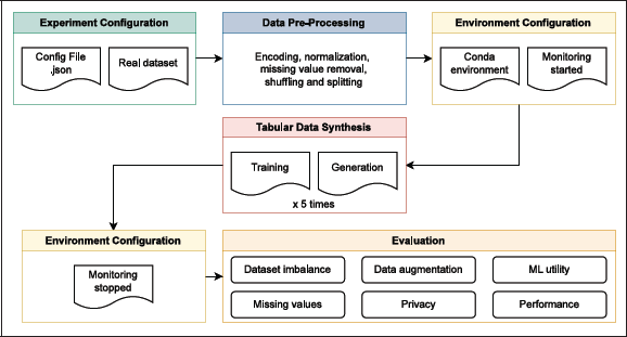
Figure 2
Overview of the benchmark architecture, which automates configuration and analysis, ensuring reproducibility and consistency across tools and datasets.
Reproducibility is ensured by organizing each tool’s folder to include the original author code (modified only for path corrections or package updates), a runtool.py script for dataset generation, and a requirements.txt file listing necessary packages.
4 Results and Discussion
This section presents the evaluation results for each test in Table 3. The six evaluation dimensions include what we consider the key challenges TDS tools must overcome to produce satisfactory synthetic data: (i) capturing real dataset characteristics with class imbalance and missing values, (ii) generating realistic data points, (iii) avoiding direct replication of existing data, (iv) preserving data quality for downstream applications, and (v) ensuring generation time and resource usage are practical for end users. These challenges are based on two main aspects: accurate replication of column distributions and preservation of inter-column correlations. We first discuss these aspects.
4.1 Correlations
Relationships between columns are essential for structural integrity and accurate downstream tasks like predictive modeling. We used the Correlation Difference metric, which we calculate as in Correlations, where we first choose randomly column pairs in the dataset (always the same pairs for all experiments), identify from the configuration what type of columns they are, and calculate their correlation. For continuous columns, we use Pearson’s correlation; for binary categorical, we use the Point-Biserial; and for all other columns, we use Spearman and Kendall. All of them use the functions from the SciPy library. For all experiments which converged, we calculate the difference between the correlations of the original dataset’s column-pairs and the correlation of the synthetic datasets.
Figure 3 shows correlation preservation, with scores normalized from zero (perfect preservation) to one (worst performance). Empty cells are cases where no dataset was generated, mainly due to: (i) PrivBayes not supporting continuous target columns (making it unsuitable for regression use cases) (Zhang et al., 2017), or (ii) tools running out of resources, reflecting typical end-user hardware constraints.
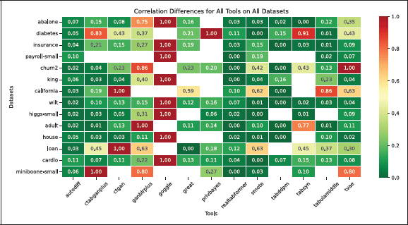
Figure 3
Heatmap showing the correlation difference for various TDS tools and use cases, where zero indicates perfect preservation of inter-column correlations, and one represents the maximum difference. Empty cells denote cases where no dataset was generated due to intentional resource constraints.
Only AutoDiff, REaLTabFormer, SMOTE, and TVAE converged for all use cases, with AutoDiff and REaLTabFormer consistently preserving correlations. GAN-based tools (CTAB-GAN+, CTGAN, GANBLR++) struggled with datasets having many columns, often failing to converge or preserve correlations. GOGGLE (Graph Neural Networks) did not converge with any of the datasets using prosumer hardware, further discussed in subsequent evaluations. Notably, SMOTE and TVAE show low correlation errors, despite their relative simplicity.
To ensure fair comparisons, PrivBayes and GOGGLE were excluded from further evaluations. The remaining seven datasets, where all tools converged (abalone, diabetes, insurance, churn2, wilt, adult, cardio), were used for analysis. PrivBayes was separately assessed for classification tasks without continuous target columns to evaluate Bayesian Networks-based tools.
4.2 Column distributions
Preserving column-wise distributions is critical in TDS and closely related to the Privacy vs. Utility trade-off (Park et al., 2018), which describes the challenge of generating useful synthetic data for its original task while protecting sensitive information. Accurate column-wise distributions ensure that the synthetic dataset retains the statistical properties of individual columns, maintaining its utility.
We compared synthetic and real column distributions using visual inspection and quantitative metrics to assess how the tool captures the original statistical characteristics. Section 4.6 then analyzes privacy, the second part of the trade-off. Figure 4 shows one of the distribution plots used for visual inspection, showing how different tools replicate column-wise distributions across datasets. Visual inspection offers an intuitive initial check of whether synthetic data captures key characteristics. This assessment was performed for all datasets and tools, with plots available in Github Repository.
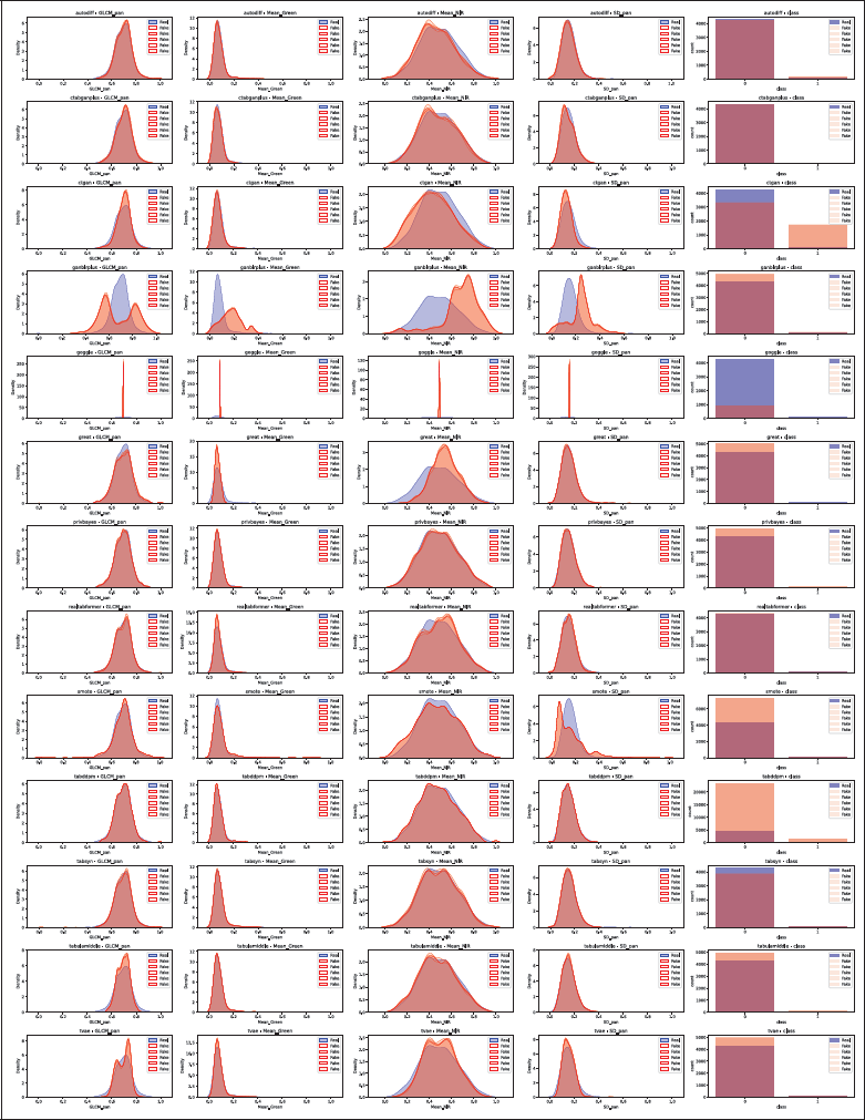
Figure 4
Distribution comparison for Wilt, with one row per TDS tool. For continuous columns, real data is in blue and synthetic in red. For categorical columns, bars show class counts with real data in blue and synthetic in red. The five synthetic distributions occasionally overlap completely. GOGGLE collapsed and therefore shows exploding densities.
Figure 4 presents plots for continuous and categorical columns. For continuous columns, real distributions are shown in blue and synthetic in red, showing whether tools capture column characteristics without assuming simple distributions like the Gaussian. For categorical columns, bar graphs display class counts, with real classes in blue and synthetic in red, making it easy to compare the number of classes and class proportions. For example, one can easily identify how GOGGLE collapses and reaches extremely high density values.
While visual inspection is a helpful starting point, it is inherently subjective and may overlook subtle discrepancies. To ensure consistency and precision, we used quantitative metrics such as the Wasserstein Distance for continuous data and Jensen–Shannon Divergence for categorical data. These metrics provide objective, numerical evaluations, capturing subtle differences in distributions that visual methods might miss, such as slight shifts in central tendency or variability. Quantitative metrics are essential for scalable and reproducible benchmarking, with results detailed in the following sections.
4.3 Dataset imbalance
Dataset imbalance is a key challenge in synthetic data generation (Davila et al., 2025), and it occurs when certain classes significantly outnumber others, potentially biasing predictive models toward dominant classes. To evaluate how well tools address this challenge, we used the metrics Wasserstein Distance (WD), Kolmogorov–Smirnov (KS) Statistic, Jensen–Shannon (JS) Divergence, and Kullback–Leibler (KL) Divergence, as implemented in the Python package (SciPy, 2024a, b, c, d).
For continuous columns, WD measures the cost of transforming one distribution into another, indicating how well tools maintain class proportions without distorting statistical properties. KS statistic captures the maximum difference between cumulative distribution functions (CDFs), reflecting alignment between real and synthetic class distributions.
For categorical data, JS Divergence measures the similarity between real and synthetic class probability distributions, with smaller values indicating better alignment. KL Divergence evaluates information loss when approximating distributions, penalizing deviations from target class balance. Percentage Class Count Difference provides an intuitive measure of relative class count differences between real and synthetic datasets.
Table 5 presents the evaluation results, with zero as the ideal value for all metrics. Top results are bolded and underlined. Each metric was calculated across all datasets for each tool, repeated five times for statistical significance, averaged, and normalized using Min–Max scaling for comparison.
Table 5
Dataset imbalance evaluation for all tools, averaged across datasets and normalized using Min–Max scaling, highlighting the top-performing tools (SMOTE, REalTabFormer, and TabSyn).
| TOOL | WASSERSTEIN DISTANCE | KS STATISTIC | CORRELATION DIFFERENCE | JS DIVERGENCE | KL DIVERGENCE | PERCENTAGE COUNT DIFFERENCE |
|---|---|---|---|---|---|---|
| AutoDiff | 0.218 | 0.164 | 0.146 | 0.211 | 0.134 | 0.154 |
| CTAB-GAN+ | 0.324 | 0.416 | 0.265 | 0.344 | 0.335 | 0.117 |
| CTGAN | 0.286 | 0.482 | 0.308 | 0.382 | 0.411 | 0.528 |
| GANBLR++ | 0.692 | 0.748 | 0.542 | 0.714 | 0.659 | 0.489 |
| GReaT | 0.576 | 0.674 | 0.209 | 0.653 | 0.189 | 0.246 |
| REalTabFormer | 0.113 | 0.294 | 0.041 | 0.185 | 0.138 | 0.002 |
| SMOTE | 0.063 | 0.062 | 0.176 | 0.015 | 0.019 | 0.198 |
| TabDDPM | 0.344 | 0.325 | 0.053 | 0.294 | 0.276 | 0.861 |
| TabSyn | 0.040 | 0.128 | 0.324 | 0.094 | 0.109 | 0.176 |
| TabuLaMiddle | 0.513 | 0.641 | 0.183 | 0.588 | 0.201 | 0.233 |
| TVAE | 0.317 | 0.543 | 0.327 | 0.423 | 0.346 | 0.414 |
The top-performing tool was SMOTE, followed by CTAB-GAN+ and TabDDPM. As expected, SMOTE performed well because it directly oversamples minority classes by interpolating between similar points, making it ideal for dataset imbalance. However, this can risk creating synthetic samples that are too similar or reinforce linear patterns, as presented in (Brandt and Lanzén, n.d.) and evidenced in the further dimensions of this benchmark. In contrast, CTGAN and GANBLR++ produce relatively lower metrics, possibly because GAN models can have difficulty capturing minority classes due to mode collapse, where the generator fails to learn the minor classes’ full distribution.
4.4 Dataset augmentation
Dataset augmentation is also a primary use case for synthetic data (Davila et al., 2025), where users expand datasets to improve model robustness and generalization by generating new data points that preserve the original dataset’s statistical properties while enhancing diversity.
To evaluate how well a tool augments the data, we used again WD, KS Statistic, and correlation differences for continuous columns, but additionally Quantile Comparison, and JS Divergence with Percentage Number of Classes Difference for categorical columns. Quantile Comparison ensures synthetic data reproduces the original data’s spread across quantiles, crucial for maintaining variability and improving model robustness. Percentage Number of Classes Difference measures whether the synthetic data retains the original number of classes, with lower values indicating better representation.
Table 6 summarizes the results, where lower values represent better performance. Top results are bold and underlined. Metrics were calculated across all datasets for each tool, repeated five times for statistical significance, averaged, and normalized using Min–Max scaling for comparison.
Table 6
Augmentation evaluation results for all tools averaged across datasets and normalized using Min–Max scaling. The top-performing tools: TabSyn, SMOTE, REalTabFormer, and TabDDPM.
| TOOL | WASSERSTEIN DISTANCE | KS STATISTIC | CORRELATION DIFFERENCE | QUANTILE COMPARISON | JS DIVERGENCE | PERCENTAGE NUMBER CLASSES DIFFERENCE |
|---|---|---|---|---|---|---|
| AutoDiff | 0.218 | 0.164 | 0.146 | 0.197 | 0.211 | 0.028 |
| CTAB-GAN+ | 0.324 | 0.416 | 0.265 | 0.287 | 0.344 | 0.045 |
| CTGAN | 0.286 | 0.416 | 0.265 | 0.226 | 0.382 | 0.014 |
| GANBLR++ | 0.692 | 0.748 | 0.542 | 0.670 | 0.714 | 0.096 |
| GReaT | 0.576 | 0.674 | 0.209 | 0.543 | 0.653 | 0.245 |
| REalTabFormer | 0.113 | 0.294 | 0.041 | 0.092 | 0.185 | 0.021 |
| SMOTE | 0.063 | 0.062 | 0.176 | 0.071 | 0.015 | 0.126 |
| TabDDPM | 0.344 | 0.325 | 0.053 | 0.259 | 0.294 | 0.006 |
| TabSyn | 0.040 | 0.128 | 0.324 | 0.066 | 0.094 | 0.123 |
| TabuLaMiddle | 0.513 | 0.641 | 0.183 | 0.465 | 0.588 | 0.332 |
| TVAE | 0.317 | 0.543 | 0.327 | 0.287 | 0.423 | 0.069 |
The top-performing tools were TabSyn, SMOTE, TabDDPM, and REalTabFormer. Unlike class imbalance handling, effective augmentation requires generating a diverse set of new samples that not only maintain statistical fidelity but also introduce meaningful variation. This is particularly captured by the Quantile Comparison metric, which evaluates how well tools reproduce the distributional spread across quantiles, a key aspect for improving model generalization. TabSyn showed the top performance on this metric, suggesting it effectively balances variability and structure. SMOTE and REalTabFormer followed closely, indicating that both sampling-based and Transformer-based methods can successfully generate data that enhances diversity while preserving core statistical properties. In the classification-only assessment, PrivBayes achieved the highest Percentage Number of Classes Difference. Simpler tools like CTGAN and TVAE perform well on basic metrics but struggle with complex distributions, supporting what is seen in Figure 4.
4.5 Missing values
Handling missing values is a key challenge in synthetic data generation. Missing values can distort analyses and degrade model performance by introducing gaps in the data. We evaluated tool performance by introducing 5%, 10%, and 20% missing values into the datasets and assessing their ability to maintain the integrity of continuous and categorical variables. For continuous columns, we used WD, KS statistic, correlation differences, and Quantile Comparison. For categorical columns, we used JS Divergence, Percentage Class Count Difference, and Percentage Number of Classes Difference, which ensures class diversity is not artificially altered when missing values affect certain classes.
Only 10 tools were evaluated, excluding GOGGLE and GANBLR++ due to poor initial performance, and TabDDPM due to errors with missing data in the configuration files. A visual inspection, shown in Figure 5, highlights the effect of missing values on the distributions of the diabetes dataset (Kahn, n.d.). Continuous plots display real distributions in blue, with red, green, and orange for synthetic datasets generated with 5%, 10%, and 20% missing values. Categorical bar plots show real classes in blue, with synthetic classes in red, green, and orange. The first column, SkinThickness, follows a multimodal distribution.
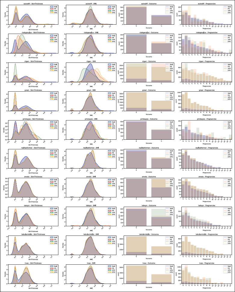
Figure 5
Distribution comparison for the Diabetes dataset, with 5%, 10% and 20% missing values. The real data distribution is plotted in blue, and synthetic data in red, green and orange. Continuous columns as density plots and categorical columns as bar plots.
Tools, such as AutoDiff, REaLTabFormer, SMOTE, TabSyn, and TabuLa, replicated distributions with minimal deviations, regardless of missing values. In contrast, CTGAN struggled, with deviations increasing as missing values rose, and it failed to preserve class proportions. CTAB-GAN+ captured simpler distributions but missed the multimodal nature of SkinThickness.
Metrics were calculated across all datasets for each tool at 5%, 10%, and 20% missing values, with evaluations repeated five times for statistical significance. Results were averaged and normalized using Min–Max scaling for fair comparison. Table 7a, 7b, and 7c show the detailed results. SMOTE demonstrated the highest robustness, maintaining stable performance across all metrics and missing value levels. AutoDiff, REaLTabFormer, TabSyn, and TabuLa also maintained acceptable performance at 20% missing values, while other tools struggled with higher levels of missing data.
Table 7
Missing-values evaluation results normalized using Min–Max scaling.
| TOOL | WASSERSTEIN DISTANCE | KS STATISTIC | CORRELATION DIFFERENCE | QUANTILE COMPARISON | JS DIVERGENCE | KL DIVERGENCE | PERCENTAGE COUNT DIFFERENCE | PERCENTAGE NUM CLASSES DIFFERENCE |
|---|---|---|---|---|---|---|---|---|
| (a) 5% Missing Values | ||||||||
| AutoDiff | 0.249 | 0.178 | 0.621 | 0.194 | 0.399 | 0.051 | 0.089 | 0.000 |
| CTAB-GAN+ | 0.412 | 0.412 | 0.217 | 0.408 | 0.420 | 0.545 | 0.019 | 0.093 |
| CTGAN | 0.829 | 0.930 | 0.669 | 0.855 | 0.846 | 0.879 | 0.722 | 0.061 |
| GReaT | 0.744 | 0.681 | 0.578 | 0.731 | 0.843 | 0.091 | 0.498 | 0.138 |
| REalTabFormer | 0.251 | 0.402 | 0.121 | 0.278 | 0.460 | 0.560 | 0.004 | 0.147 |
| SMOTE | 0.061 | 0.072 | 0.182 | 0.062 | 0.048 | 0.051 | 0.376 | 0.000 |
| TabSyn | 0.074 | 0.112 | 0.418 | 0.052 | 0.123 | 0.030 | 0.045 | 1.000 |
| TabuLaMiddle | 0.362 | 0.438 | 0.091 | 0.401 | 0.531 | 0.018 | 0.452 | 0.055 |
| TVAE | 0.830 | 0.879 | 0.378 | 0.835 | 0.842 | 0.422 | 0.478 | 0.186 |
| (b) 10% Missing Values | ||||||||
| AutoDiff | 0.368 | 0.182 | 0.642 | 0.319 | 0.415 | 0.074 | 0.069 | 0.000 |
| CTAB-GAN+ | 0.798 | 0.605 | 0.471 | 0.799 | 0.635 | 0.669 | 0.147 | 0.092 |
| CTGAN | 0.725 | 0.963 | 0.523 | 0.753 | 0.872 | 0.875 | 0.734 | 0.034 |
| GReaT | 0.753 | 0.711 | 0.583 | 0.735 | 0.887 | 0.077 | 0.495 | 0.167 |
| REalTabFormer | 0.269 | 0.436 | 0.108 | 0.263 | 0.469 | 0.531 | 0.004 | 0.165 |
| SMOTE | 0.067 | 0.065 | 0.181 | 0.029 | 0.043 | 0.047 | 0.368 | 0.000 |
| TabSyn | 0.072 | 0.092 | 0.000 | 0.038 | 0.067 | 0.075 | 0.042 | 0.000 |
| TabuLaMiddle | 0.348 | 0.398 | 0.098 | 0.382 | 0.384 | 0.015 | 0.437 | 0.097 |
| TVAE | 0.735 | 0.984 | 0.537 | 0.789 | 0.804 | 0.399 | 0.459 | 0.261 |
| (c) 20% Missing Values | ||||||||
| AutoDiff | 0.405 | 0.184 | 0.589 | 0.385 | 0.386 | 0.058 | 0.081 | 0.000 |
| CTAB-GAN+ | 0.378 | 0.442 | 0.288 | 0.419 | 0.420 | 0.356 | 0.031 | 0.092 |
| CTGAN | 0.911 | 1.000 | 0.662 | 0.976 | 0.925 | 0.904 | 0.732 | 0.042 |
| GReaT | 0.769 | 0.678 | 0.563 | 0.782 | 0.863 | 0.071 | 0.501 | 0.129 |
| REalTabFormer | 0.267 | 0.435 | 0.128 | 0.336 | 0.492 | 0.433 | 0.005 | 0.138 |
| SMOTE | 0.049 | 0.082 | 0.162 | 0.071 | 0.051 | 0.049 | 0.378 | 0.000 |
| TabSyn | 0.502 | 0.972 | 0.231 | 0.533 | 0.835 | 0.061 | 0.021 | 0.033 |
| TabuLaMiddle | 0.334 | 0.411 | 0.116 | 0.406 | 0.466 | 0.520 | 0.451 | 0.057 |
| TVAE | 0.647 | 0.893 | 0.303 | 0.658 | 0.750 | 0.311 | 0.479 | 0.148 |
4.6 Privacy
Another key aspect of the Privacy vs. Utility trade-off is assessing how closely synthetic data resembles real data while ensuring privacy. This is crucial when real datasets contain sensitive or personally identifiable information. Synthetic data offers an alternative to traditional anonymization methods like masking, which often cause significant information loss. The challenge is to generate data that is useful for downstream tasks without exposing individual records.
We evaluated privacy using Distance to Closest Record (DCR) (Hernandez et al., 2022; Park et al., 2018) and Nearest Neighbor Distance Ratio (NNDR) (Zhao et al., 2024). DCR measures the Euclidean distance between each synthetic record and its nearest real counterpart. Lower DCR values enhance utility but increase privacy risk, while higher values suggest better privacy at the cost of utility. NNDR compares the distance between a synthetic record and its closest real record to its second-closest synthetic record, with higher values indicating better privacy protection through greater dispersion.
Table 8 summarizes the results, where higher values indicate stronger privacy protection. Top-performing tools are bolded and underlined. Each metric was calculated across all datasets and tools, repeated five times for statistical reliability, averaged, and normalized using Min-Max scaling for comparison.
Table 8
Privacy results for all tools averaged across datasets and normalized using Min-Max scaling, highlighting the top-performing tools (CTAB-GAN+, REalTabFormer, and TabDDPM). The best score is one, and the worst is zero.
| TOOL | DISTANCE TO CLOSEST RECORD | NEAREST NEIGHBOR DISTANCE RATIO |
|---|---|---|
| AutoDiff | 0.162 | 0.847 |
| CTAB-GAN+ | 0.139 | 0.870 |
| CTGAN | 0.230 | 0.844 |
| GReaT | 0.046 | 0.751 |
| REalTabFormer | 0.283 | 0.781 |
| SMOTE | 0.032 | 0.342 |
| TabSyn | 0.261 | 0.750 |
| TabDDPM | 0.329 | 0.810 |
| TabuLaMiddle | 0.062 | 0.438 |
| TVAE | 0.101 | 0.837 |
TabDDPM, CTAB-GAN+, and REalTabFormer performed best in privacy. Despite its strong performance in previous evaluations, SMOTE underperformed in privacy, generating data points too similar to the original, demonstrating a poor Privacy vs. Utility trade-off. In contrast, CTGAN achieved high privacy scores but struggled with column distributions and correlations, also demonstrating the trade-off.
Tools like PrivBayes allow configurable parameters such as the privacy budget (𝜖), which controls the trade-off between utility and privacy under Differential Privacy (DP). DP adds controlled noise to ensure that including or excluding any single record does not significantly affect outputs, offering strong privacy guarantees. However, evaluating DP mechanisms is beyond the scope of this benchmark.
4.7 Machine learning utility
Machine learning (ML) Utility evaluates how well synthetic datasets replace real ones in training ML models for classification and regression tasks. To assess ML Utility, we used nine classifiers and four regressors, as shown in Table 9. Models were tested on real data to measure predictive accuracy and robustness. The metrics included Accuracy, AUC, and F1 Score (micro, macro, weighted) for classification, and EVS, MAE, and R2 for regression (Pedregosa et al., 2011). Accuracy measures overall correctness, AUC assesses class separation, and F1 Score balances precision and recall. EVS captures target variability, MAE measures average error, and R2 indicates the proportion of variance explained by the model.
Table 9
Classifiers and regressors used for the ML utility evaluation.
| CLASSIFICATION METHODS | REGRESSION METHODS |
|---|---|
| Decision Trees | Bayesian Ridge Regression |
| Gaussian Naive Bayes (NB) | Lasso Regression |
| K-Nearest Neighbors (KNN) | Linear Regression |
| Linear Support Vector Machine (SVM) | Ridge Regression |
| Logistic Regression | |
| Multilayer Perceptron (MLP) | |
| Perceptron | |
| Random Forest | |
| Radial Support Vector Machine (SVM) |
Table 10 presents the results as differences between model performance on real and synthetic data. Zero means equal performance, positive values favor real data, and negative values favor synthetic data. For MAE, lower values are better, so its inverse is shown for consistency. While accuracy and F1 Micro appear similar, accuracy measures overall correctness, while F1 Micro accounts for class imbalance. Similarly, EVS focuses on variability, while R2 also penalizes systematic prediction errors.
Table 10
ML utility results showing the difference between the model’s performance trained with real datasets and trained with synthetic datasets. For all metrics, if the difference is negative, the model performed better with synthetic data than with real data. If the difference is positive, the model performed worse.
| TOOL | ACCURACY | AUC | F1 MICRO | F1 MACRO | F1 WEIGHTED | EVS | INVERSE MAE | R2 SCORE |
|---|---|---|---|---|---|---|---|---|
| AutoDiff | –0.072 | 0.010 | –0.070 | –0.009 | –0.080 | 0.038 | 0.009 | 0.062 |
| CTAB-GAN+ | –0.052 | 0.074 | –0.046 | 0.071 | 0.053 | 0.176 | 0.145 | 0.172 |
| CTGAN | 0.089 | 0.046 | 0.081 | 0.053 | 0.093 | 0.193 | 0.472 | 0.192 |
| GANBLR++ | 0.118 | 0.152 | 0.121 | 0.156 | 0.137 | 0.548 | 0.342 | 0.546 |
| GReaT | 0.043 | 0.051 | 0.040 | 0.070 | 0.033 | 0.395 | 0.398 | 0.665 |
| REalTabFormer | –0.024 | –0.029 | –0.020 | –0.028 | –0.023 | 0.003 | –0.026 | 0.003 |
| SMOTE | –0.011 | –0.014 | –0.013 | –0.017 | –0.016 | 0.143 | 0.028 | 0.145 |
| TabDDPM | 0.019 | –0.031 | 0.017 | –0.023 | 0.010 | 0.034 | 0.182 | 0.035 |
| TabSyn | –0.046 | –0.041 | –0.043 | –0.040 | –0.078 | 0.018 | –0.035 | 0.017 |
| TabuLaMiddle | –0.063 | –0.072 | –0.059 | –0.052 | –0.080 | 0.204 | 0.066 | 0.011 |
| TVAE | –0.024 | –0.015 | –0.021 | –0.006 | –0.025 | 0.210 | 0.159 | 0.346 |
Table 10 shows that AutoDiff, TabuLa, REalTabFormer, and TabSyn preserve ML utility better. In general, tools perform better in classification than in regression, likely because the discrete nature of classification targets is easier to learn. SMOTE presented a strong classification performance; however, it is closely similar to the real data, which suggests limited record variability.
4.8 Computational performance
Computational performance measures the resource usage and execution speed during synthetic data generation, assessing computational efficiency and practical usability across tools. Advanced tools, such as deep learning-based models, often rely on GPUs, while simpler methods like PrivBayes and SMOTE prioritize lightweight execution without specialized hardware. This comparison highlights whether complex tools justify their resource demands with superior results in other dimensions (e.g., dataset balancing, or ML utility).
Table 11 shows the results for CPU, GPU, and memory usage, as well as runtime, measured by the mean, max, and standard deviation across five runs for all tools and datasets.
Table 11
Performance results for all tools averaged across datasets. Top-performing tools are SMOTE and PrivBayes; REalTabFormer shows the longest runtime and high resource usage.
| TOOL | MEAN CPU (%) | MAX CPU (%) | MEAN MEMORY (%) | MAX MEMORY (%) | MEAN GPU (%) | MAX GPU (%) | RUNTIME (S) |
|---|---|---|---|---|---|---|---|
| AutoDiff | 14 | 24 | 15 | 16 | 7 | 37 | 3240 |
| CTAB-GAN+ | 18 | 28 | 7 | 8 | 34 | 56 | 863 |
| CTGAN | 13 | 59 | 13 | 25 | 32 | 36 | 572 |
| GANBLR++ | 27 | 88 | 16 | 19 | 0 | 0 | 1790 |
| GOGGLE | 45 | 56 | 23 | 24 | 0 | 0 | 1106 |
| GReaT | 9 | 22 | 13 | 14 | 77 | 86 | 3714 |
| PrivBayes | 17 | 32 | 18 | 19 | 0 | 0 | 106 |
| REalTabFormer | 10 | 37 | 21 | 39 | 28 | 77 | 7682 |
| SMOTE | 25 | 38 | 17 | 17 | 0 | 0 | 248 |
| TabDDPM | 11 | 36 | 19 | 20 | 20 | 31 | 666 |
| TabSyn | 17 | 25 | 19 | 22 | 13 | 57 | 317 |
| TabuLaMiddle | 25 | 33 | 23 | 23 | 76 | 90 | 1097 |
| TVAE | 12 | 90 | 17 | 22 | 13 | 15 | 465 |
PrivBayes is the most resource-efficient tool (106s runtime, 17% CPU, no GPU), while SMOTE (248s, 25% CPU, no GPU) is the best for mixed data. REalTabFormer has the highest runtime (7682s) with high memory (21% mean, 39% max) and GPU usage (28% mean, 77% max), reflecting its complex architecture.
GOGGLE and GANBLR++ show high resource demands due to graphical modeling, with GOGGLE using 45% CPU and GANBLR++ peaking at 88% CPU.
GAN models like CTAB-GAN+ balance efficiency and runtime (863s, 18% CPU, 7% memory), while Transformer models (REalTabFormer, TabuLa) are resource-intensive, with TabuLa reaching 90% GPU usage. Diffusion-based TabDDPM offers balanced performance (11% CPU, 19% memory, 666s runtime). Hybrid models TabSyn (317s runtime, 17% CPU, 19% memory) and AutoDiff (14% CPU, 15% memory) provide efficient resource usage with minimal GPU reliance, maintaining strong performance across evaluations.
4.9 Aggregated benchmark results and discussion
We aggregated the results per model type across the six evaluation dimensions. Metrics were normalized, averaged per tool, and re-normalized to a 1–10 scale, where 10 means best performance, and 1 represents poor performance or failed use cases.
We assigned equal weight to all metrics within each of the six dimensions, aiming to provide general, comparable conclusions across models. We acknowledge that alternative weighting could be applied, depending on the priorities of specific use cases. Figure 6 compares the different TDS model types, using these normalized scores to provide a consolidated view of their overall strengths and limitations.
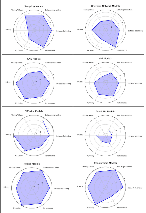
Figure 6
Spider web diagram summarizing model performance across the six benchmark dimensions. The scores are calculated by aggregating each dimension and are scaled 1–10.
Sampling models like SMOTE excel in handling imbalance, augmentation, and missing values, with top resource efficiency, making them ideal for fast, lightweight data synthesis. However, their low variability affects ML utility and privacy, as they often generate data too close to the original. While this limits their use in privacy-sensitive or high-variability tasks, their simplicity and low computational demands make them accessible for users with limited hardware, especially for balancing and augmentation needs in large datasets.
Graph Neural Networks (GNNs) like GOGGLE and GANBLR++ perform poorly with our prosumer setup, often failing to converge without high-performance clusters. Their reliance on complex graphical structures introduces computational overhead, making them unsuitable for prosumer hardware. They were still shown in Figure 6 for completeness, but the dimensions where they were excluded were left blank, since the results are not comparable. This is also the case for PrivBayes, which shows that Bayesian Networks are highly efficient, with strong privacy and performance scores, but their limited ability to model complex relationships affects their results for dataset augmentation and balancing, making them better suited for privacy-prioritized applications.
GAN-based models such as CTGAN and CTAB-GAN+ deliver moderate performance, excelling in augmentation and imbalance handling but struggling with missing values and privacy. Despite these challenges, GANs generate realistic synthetic data, provided the data is complete and pre-processed. Diffusion models achieve consistently high scores across all dimensions, balancing privacy, utility, and performance, but require significant tuning and resources for optimal use. Finally, Hybrid and Transformer models stand out with high scores in augmentation, missing values, and ML utility. Transformers (e.g., REaLTabFormer, TabuLa) deliver excellent results but demand substantial computational resources, reflecting their complexity. Hybrid models (e.g., AutoDiff, TabSyn) combine strengths from multiple models, offering balanced, efficient performance suitable for diverse use cases, making them versatile tools for most TDS applications.
4.10 Discussion on hyperparameter tuning
The experiments above were carried out, as mentioned in Section 3, using the parameters tuned by the original authors, without performing additional hyperparameter tuning. We chose this approach to avoid researcher bias and to benchmark the tools in their out-of-the-box configuration.
However, complex TDS models benefit greatly when their hyperparameters are tuned for each dataset. Simple TDS tools, such as SMOTE and PrivBayes, require no hyperparameter tuning because they rely on fixed algorithmic procedures rather than parameterized learning processes. In contrast, GANs are well known to be unstable during training, meaning that key hyperparameters, such as learning rates, optimizer choice, gradient penalty, and batch size, can cause training to collapse or oscillate. (Arjovsky, Chintala, and Bottou, 2017; Mescheder, Geiger, and Nowozin, 2018) For this reason, GAN-based tools typically incorporate stabilization techniques, such as Wasserstein loss or spectral normalization, which should not be, or only very carefully, altered.
Diffusion models, on the other hand, are much more stable to train because their training is explicit likelihood-based, as shown in Figure 1. Yet, their effectiveness is sensitive to the chosen hyperparameters (Kotelnikov et al., 2023), such as the number of diffusion steps, learning rate, or noise schedule. As a result, hyperparameter tuning can significantly improve the performance of diffusion-based models. The situation is similar for Transformer-based tools, which depend heavily on their hyperparameters (Casola, Lauriola, and Lavelli, 2022), such as number of layers, hidden dimension, number of attention heads, or learning rate schedules.
This study acknowledges that a further benchmark including hyperparameter tuning would increase fairness toward certain models, such as Diffusion or Transformers, which are capable of producing superior results when properly tuned. Nevertheless, Diffusion, Transformer-based, and Hybrid models already achieved better performance in our benchmark with respect to correlations and distributions, which are the basis of synthetic data quality. In the aggregated results, they obtained the highest scores across all dimensions, except computational performance.
We expect that including hyperparameter tuning in future experiments will further increase the quality of the generated synthetic data, but at the expense of higher computational cost. Exploring this trade-off is left for future work.
5 Conclusion
Through the evaluation across six dimensions (dataset imbalance, data augmentation, handling missing values, privacy, ML utility, and performance), we gained valuable insights into the capabilities and limitations of individual tools and models for TDS. Sampling-based tools like SMOTE demonstrated exceptional performance in dataset imbalance, augmentation, and resource efficiency, but struggled with privacy and variability. Hybrid and Transformer models stood out as the most consistent performers across all dimensions, achieving high scores in utility and privacy but requiring substantial computational resources. In contrast, GNNs and GANs combined with graphical models often failed to converge under our setup, highlighting their unsuitability for environments without access to high-performance clusters.
Our findings also emphasize the trade-offs inherent in different TDS models. Diffusion models showed promise with high scores across evaluations but were complex to configure, while Bayesian Networks offered strong privacy protection and efficiency but limited utility in dataset imbalance and augmentation tasks. VAEs, although moderate in performance, serve as the basis for high-performing Hybrid models. GANs displayed versatility in augmentation and dataset imbalance but had moderate to low privacy and utility results, indicating the need for careful consideration in sensitive use cases.
Beyond the quantitative findings, we observed additional non-functional aspects that influence tool usability. Tools like TabDDPM and TabSyn, despite their strong performance, were challenging to implement and required significant effort to configure properly. Others, such as GANBLR++ and GOGGLE, had complicated requirements and dependencies, making them time-consuming to deploy effectively. These considerations, while not easily quantifiable, are critical when selecting a TDS tool, as they directly impact the practicality and adoption of these models in real-world scenarios. Overall, this benchmark provides a detailed roadmap for researchers and practitioners to navigate the landscape of TDS tools, aligning their choices with specific needs and constraints.
This benchmark is limited by the fact that we do not perform any hyperparameter tuning for complex models, such as Diffusion or Transformers, which may impact their effectiveness. Our future work includes experiments with hyperparameter tuning (Davila, Turaev, and Wingerath, 2025).
Appendices
Appendix A: Library Versions in the Experiments
For the sake of reproducibility and software versioning, we add the package requirements for each of the TDS tools used in this experiment.
Table 12
TDS tools and required packages.
| TDS TOOL | PACKAGE REQUIREMENTS |
|---|---|
| SMOTE | pandas==2.2.2, numpy==2.0.0, scikit-learn==1.5.2, imbalanced-learn==0.13.0 |
| PrivBayes | diffprivlib==0.6.3, dill==0.3.7, dython==0.6.8, joblib==1.2.0, lifelines==0.27.8, matplotlib==3.7.2, numpy==1.26.0, pandas==1.3.4, pyjanitor==0.26.0, pandas_flavor==0.6.0, scikit_learn==1.3.0, scipy==1.11.3, seaborn==0.13.0, thomas_core==0.1.3, synthetic-data-generation, torch, gpustat |
| CTGAN | tqdm==4.66.5, torch==2.1.0, numpy==2.0.0, pandas==2.2.2, scikit-learn==1.5.2, ctgan, joblib==1.4.2, rdt==1.7.0 |
| CTAB-GAN+ | numpy==1.21.0, torch==1.10.0+cu113, torchvision==0.11.1+cu113, torchaudio==0.10.0+cu113, pandas==1.2.1, scikit-learn==0.24.1, dython==0.6.4.post1, scipy, gpustat, tqdm, -f https://download.pytorch.org/whl/torch_stable.html |
| GANBLR++ | ganblr |
| TVAE | tqdm==4.66.5, torch==2.1.0, numpy==2.0.0, pandas==2.2.2, scikit-learn==1.5.2, ctgan, joblib==1.4.2, rdt==1.7.0 |
| TabDDPM | catboost==1.0.3, category-encoders==2.3.0, dython==0.5.1, icecream==2.1.2, libzero==0.0.8, numpy==1.21.4, optuna==2.10.1, pandas==1.3.4, pyarrow==6.0.0, rtdl==0.0.9, scikit-learn==1.0.2, scipy==1.7.2, skorch==0.11.0, tomli-w==0.4.0, tomli==1.2.2, tqdm==4.62.3 |
| GOGGLE | chardet==5.1.0, cvxpy==1.1, dgl==0.9.0, geomloss==0.2.5, matplotlib==3.7.0, numpy==1.23.0, packaging==21.3, pandas==1.4.3, pgmpy==0.1.21, scikit-learn==1.1.1, seaborn==0.12.2, synthcity==0.2.2, torch==1.12.0, torch-geometric==2.2.0, torch-sparse==0.6.16, torch_scatter==2.1.0 |
| GReaT | datasets≥2.5.2, numpy≥1.23.1, pandas≥1.4.4, scikit_learn≥1.1.1, torch≥1.10.2, tqdm≥4.64.1, transformers≥4.22.1, accelerate≥0.20.1 |
| REalTabFormer | torch, bandit≥1.6.2,<2.0, black~=22.0, build~=0.9.0, import-linter[toml]==1.2.6, openpyxl~=3.0.10, pre-commit≥2.9.2,<3.0, pylint≥2.5.2,<3.0, pytest-cov~=3.0, pytest-mock≥1.7.1,<2.0, pytest-xdist[psutil]~=2.2.1, pytest~=6.2, trufflehog~=2.1, twine~=4.0.1, pandas, datasets, scikit-learn, transformers, realtabformer |
| TabuLa | datasets≥2.5.2, numpy≥1.24.2, pandas≥1.4.4, scikit_learn≥1.1.1, torch≥1.10.2, tqdm≥4.64.1, transformers≥4.22.1 |
| AutoDiff | numpy==2.0.0, pandas==2.2.2, scikit-learn==1.5.2, scipy==1.10.1, torch==2.1.0, gpustat==1.0.0, psutil==5.9.4, tqdm==4.65.0, ipywidgets==7.8.5, jupyter==1.0.0, matplotlib==3.7.1 |
| TabSyn | numpy==2.0.0, pandas==2.2.2, scikit-learn==1.5.2, scipy==1.10.1, torch==2.1.0, icecream==2.1.2, category_encoders==2.3.0, imbalanced-learn==0.14.0, transformers==4.25.0, datasets==2.8.0, openpyxl==3.1.2, xgboost==1.7.5 |
Competing Interests
The authors have no competing interests to declare.
Author Contributions
Maria Davila was the main contributor to this work. She carried out the experiments and designed the methodology, playing a central role in the conception and execution of the study.
Benjamin Wollmer contributed to the design of the evaluation process and participated in the critical review of the proposed method, ensuring its robustness and relevance.
Fabian Panse was responsible for the technical correctness of the benchmark and implementation of the data synthesis tools, contributing significantly to the reproducibility and reliability of the results.
Wolfram Wingerath served as the supervising professor. He ensured the scientific validity of the methodology, evaluation, and writing process and provided guidance throughout the development of the work.