
1 Introduction
Data-intensive approaches, pertaining to machine learning and artificial intelligence, have been widely applied in addressing air pollution problems. Typical examples include data clustering and association rule mining methods, which have found applications in different settings (Soares et al., 2023; Wu, Wen and Zhu, 2024). The former, for instance, have been applied in quantifying pollution levels, particularly in remote sensing, where they have been applied to obtain ground-level concentrations of atmospheric pollutants. Examples of the application of the latter include the association of particulate matter with atmospheric levels using the measurement of one pollutant to estimate the concentration of another. However, most approaches are still hampered by model optimisation challenges that derive from inherent randomness in spatio-temporal and sectoral data variations. A standard approach to address data randomness hinges on the concepts of data harmonisation (Cheng et al., 2024; Diaz-de Arcaya et al., 2025) and data augmentation (Mumuni, Mumuni and Gerrar, 2024; Wang et al., 2024). The former describes a process for resolving variations in data syntax, while the latter relates to artificially enhancing data size, diversity and other parameters in order to improve model performance. This paper proposes a novel approach to address data randomness, with built-in robust mechanisms to generate the “most parsimonious model” with a potential “global representativeness” to highlight data-driven solutions to regional and global environmental challenges. It is powered by two algorithms that sequentially estimate, maximise and optimise parameters from thirty thousand ground-level air pollution data points obtained from different locations in southern China; it generates statistical associations among the pollutants and presents interpretable visual outputs.
1.1 Purpose of Research
The main purpose of this research is to develop a data modelling method to address societal challenges, such as air pollution – a local, regional and global multi-dimensional challenge, that cuts across disciplines, sectors and regions. Despite being one of the greatest environmental threats to human health and well–being, air quality is not explicitly highlighted in the United Nation’s Sustainable Development Goals (SDG) agenda (Zusman, Elder and Sussman, 2020). It appears subtly in several SDGs, for instance, the interaction between climate change and air pollution has been reported to “amplify risks to human health and crop production” (Sillmann et al., 2021), and air pollution has been linked to respiratory and cardiovascular diseases (Mak and Ng, 2021; Newby et al., 2015; Zhang et al., 2022b). Ozone, for instance, is known to reduce crop yields, implying that addressing its spread supports food security. The above examples are related to the SDGs 1, 2, 3, 8, 9, 10 and 11. More specifically, target 11.6.2 of SDG 11 – sustainable cities and communities – focuses on reducing the environmental impact of cities by improving surrounding air quality conditions. We are therefore challenged to adopt interdisciplinary approaches to uncover the triggers of SDG indicators, by detecting information hidden in their data attributes (Mwitondi and Said, 2021; Mwitondi, Munyakazi and Gatsheni, 2018b).
Thus, the choice of air pollution data for developing and testing the method lies on the fact that “it affects, and/or is affected by, almost all the 17 SDGs”. Most importantly, the SDG epitomise all aspects of our existence and so, it is reasonable to assume that through coordinated and collaborative studies on air quality, the research community can unfold our understanding of how they interact and the impact of such interaction on our livelihood. In other words, it will help unify spatio-temporal and other global initiatives, such as the World Health Organization (WHO) air quality guidelines (WHO, 2021), United Nations Environment Programme (UNEP) reports (UNEP, 2023), and other organisations such as the Global Alliance on Health and Pollution (GAHP, 2023).The sampled dataset is assumed to reflect “global representativeness” in air pollution modelling, given China’s role on both sides of the pollution spectrum as well as the large number of environmental studies that have been carried out in the country.
1.2 Study Motivation
The motivation for this work derives from our research interest in addressing societal challenges through Big Data Modelling of Sustainable Development Goals (BDMSDG) (Mwitondi and Said, 2021; Mwitondi, Munyakazi and Gatsheni, 2020). The interactions of humans and their habitat inevitably lead to mutual impacts that often turn out to be adverse on both sides (Anser et al., 2024; Edo et al., 2024). The paper is set on the premise that human and natural activities generate large volumes of multifaceted environmental and other types of data, much faster than the rate at which the data can be processed, hence the need for developing more sophisticated, faster and more efficient data analytic tools and methods than ever before. It focuses on the applications of machine learning techniques in environmental modelling, which is a fundamental aspect of SDG. Thus, It is reasonable to assert that the motivation hinges on the complexity of SDG and the way to address them through robust data modelling methods.
1.2.1 Complexity of SDG Interactions
For an intuition into the mutual impact of human–nature interactions, consider the inherent correlations among different aspects of the 17 SDGs (United Nations, 2015). One aspect that relates to each SDG is “environmental pollution”. Thus, conducting air quality studies and spatial analyses can play an important role in planning and laying down policies for land use, infrastructural and business development, which hinge on different SDGs. For instance, if pollution hotspots in southern China (a major trading port and manufacturing hub) can be identified, preventive measures and stricter pollution abatement policies can be implemented in concerned cities or counties, so that overall pollution levels can be effectively reduced, ensuring healthy lives and promoting well–being for all citizens and visitors (SDG #3).
Air quality and climatic conditions mutually impact each other: climate change can affect air quality, and certain air pollutants can affect climate change (Feng et al., 2019) (SDG #13). Other SDGs that are closely associated with air quality include SDG #11 (Sustainable Cities and Communities), the attainment of which relates to reducing air pollution and making cities and human settlements inclusive, safe, resilient and sustainable. Smart and sustainable city development shows care and a focus on maintaining good air quality within neighbourhood levels and within various spatial scales. Focusing on a specific region, such as southern China, contributes to SDG #17 (Partnerships), which facilitates interdisciplinarity across geographical regions, legislations, infrastructural setups, and promotes citizen engagement.
1.2.2 Addressing the Complexity of SDG interactions
Recognising the complexity stated in Section 1.2.1, we adopt the mathematical concept of “non-orthogonality” of SDGs (Mwitondi, Munyakazi and Gatsheni, 2020). Different methods have been developed to track, monitor and model environmental pollution, including automated data-driven tools to capture, model and track environmental variations (Mwitondi, Munyakazi and Gatsheni, 2020). The literature on environmental pollution is awash with applications of sophisticated statistical and machine learning methods (Liu et al., 2022a; Pan, Harrou and Sun, 2023). Data–intensive, machine learning approaches have been used in the remote processing of ground-level concentrations of atmospheric pollutants such as , PM2.5 and ozones (Chi et al., 2022; Du et al., 2022; Xu et al., 2018). Clustering methods have been applied in quantifying pollution levels as well as in remote sensing (Hsu et al., 2023; Zhang and Yang, 2022). Other studies have applied temperature inversion methods (Feng, Wei and Wang, 2020), partial differential equations with appropriate initial and boundary conditions (Shafiev, 2024), as well as the use of remotely sensed datasets (Lin et al., 2020; Mak et al., 2018). A study focusing on surface and sea surface pressure, geopotential height, temperature, relative humidity, wind field, and vertical velocity, established an association between regional weather and climate events on one side and large-scale circulation anomalies on the other (Cai et al., 2020). Global studies on the relationship between economic development and pollution are also well documented (Yan et al., 2024). The main challenge of the foregoing studies revolves around model optimisation (Liu et al., 2022a; Vardoulakis et al., 2007; Zhang et al., 2022a), i.e., the need to develop “robust” methods to perform relevant tasks that can be replicated in a spatio-temporal context. Further, socio-demographic factors, coupled with economic, cultural, political, legislative and technical variations, directly affect pollution levels as well as mitigation efforts. Focusing on southern China was therefore particularly appealing due to the country’s role on both sides of the pollution spectrum, i.e., as a polluter and as a pollution mitigator (Liu et al., 2022b; Sun, 2016; Zheng and Kahn, 2017). Furthermore, most of the aforementioned studies have been carried out in China, hence associating results from a “robust” model with “acceptable metrics” such as SDG indicators and sharing the relevant datasets publicly would be a major step towards our understanding of SDG attainment (Mak and Lam, 2021; Mwitondi, Munyakazi and Gatsheni, 2020).
Our paper complements previous studies by adopting an interdisciplinary approach to spatio-temporal air pollution modelling, via the two algorithms in Section 2.2.4 that are embedded with the flexibility to run different techniques including, in this specific application, Principal Component Analysis (PCA), Cluster Analysis (Chapmann, 2017; Kogan, 2007), Correspondence Analysis (CA) (Hirschfeld, 1935), K-Means (Lloyd, 1957; MacQueen, 1967) and the Expectation-Maximisation (EM) algorithm (Dempster et al., 1977). Our main idea hinges on an interdisciplinary approach to both problem identification and solving, i.e., balancing the power of data, machine learning techniques, and underlying domain knowledge. We focus on the identification of pollution levels of different pollutants in the sampled area, then propose two algorithms for identifying spatio-temporal associations among key air pollutants. The novelty of this study derives from the role of the two algorithms, which hinges on their “robustness” in addressing data randomness and on highlighting the path towards addressing the “non-orthogonality” of SDGs, i.e., the factors that affect the extent and impact of air pollution within any geographical area are not confined to the geographical boundaries of that area. This can be better understood in the context of how our atmosphere is structured, because pollutants along the air can travel from one country to another within a short period of time, as well as across various vertical layers within the atmosphere. Table 1 describes the structured layers of our atmosphere and their relevance to humanity.
Table 1
Layers of our atmosphere.
| LAYER | DESCRIPTION & RELEVANCE TO HUMANITY |
|---|---|
| Troposphere | Closest to our habitat–stretching up to 10 km above earth. Its temperature decreases inversely with distance from the centre of the earth (approx. per kilometre) (Omrani et al., 2022). |
| Stratosphere | Consists the majority of atmospheric ozone, which absorbs ultraviolet radiation and protects us from potential health risks. It is characterised by high temperatures over summer and lowest over the winter period (Xu et al., 2023). |
| Mesosphere | The temperature varies inversely with vertical height above ground (Laštovička, 2023). |
| Thermosphere/Ionosphere | Absorption of energetic ultraviolet & X-ray radiation from the sun, thus temperature increases with vertical height. They also vary between night and day as well as between seasons. It reflects and absorbs radio waves, allowing global radio wave transmission (Goncharenko et al., 2021). |
| Exosphere | Contains mainly oxygen and hydrogen atoms, but they rarely collide - they follow “ballistic” trajectories under the influence of gravity (Janches et al., 2021). |
| Magnetosphere | The outer region surrounding the earth, where charged particles spiral along the magnetic field lines, with the earth behaving like a huge magnet (Lu et al., 2022). |
In this study, we focus on the tropospheric layer – the bottom layer of the earth’s atmosphere. It constitutes of about 75–80% of the atmospheric mass, with its temperature variation affected by height and time of day and/or year. Most of our terrestrial weather—clouds, rain, snow—derive from it, making it a particularly interesting research scope.
1.3 Research Question and Objectives
Identification of relevant data attributes and the nature of their complex interactions are fundamental to creating robust data-driven solutions. Using air pollution data, described in Table 2, this study seeks to address the following problem: Identifying optimal parameters for air pollution control by learning rules from datasets of multiple pollutants. Learning rules from data is particularly important if our data processing capabilities are to match the rate at which we generate it (Ridzuan and Zainon, 2022; Zhou et al., 2021). To address the problem, we lay down the following general and specific objectives.
Table 2
Selected key air pollutants.
| DATA ITEM | DESCRIPTION | DIMENSION & COMPLETENESS |
|---|---|---|
| (FSPMC) | Fine Suspended Particulates (FSP) | samples: missing |
| NO_2 | Nitrogen Dioxide | samples: missing |
| Nitrogen Oxides–in Hong Kong | samples: missing | |
| O_3 | Ozone | samples: missing |
| (RSPMC) | Respirable Suspended Particulates (RSP) | samples: missing |
| Time | Daily and hourly recording | From 00:00hrs to 23:00hrs of 1–31 January 2023, 1–30 April 2023, 1–31 July 2023 and 1–31 October 2023 (inclusive) |
| DayTimes | Discretised time periods of day |
|
| Period | Monthly weather periods | January, April, July and October |
To develop a robust data-driven method for air quality monitoring and control
To harmonise data from disparate air quality stations in southern China (including Hong Kong and Macau).
o clean and prepare the newly created composite dataset for large-scale modelling.
o design and test mechanisms for extracting and analysing information relevant to the research problem.
To apply the established method on datasets acquired from multiple stations in southern China (including Hong Kong and Macau)
o carry out initial exploratory data analysis to understand the general behaviour of the data.
To identify associations among data attributes like pollutants, timelines and locations.
To select and optimise key parameters and match patterns in a spatio-temporal context.
To demonstrate and assess applicability of the method across other SDG applications.
2 Methods
This section introduces data sources and techniques used in the study. The adopted methods are twofold, namely, technical and applied. From the technical perspective, we present two algorithms. One “estimates” the parameters of the pollutants and the other uses the estimates to perform comparative analysis for best model selection. The two algorithms are applied to establish optimal associations among selected air pollutants, as well as between pollutant types at discretised daily and annual time periods. From the application perspective, it hinges on improving the quality of life by addressing air pollutant trends, hence touching on several SDGs and their “non-orthogonality”.
2.1 Data Sources
Pollution datasets were collected from southern China, including Hong Kong and Macau. Data came from 272 stations that included ambient, roadside, and environmental resources monitoring units, with common collection sites including schools, monitoring sites, parks, roadside, street entrances, etc. The data covered the period 00:00hrs on 1 January 2023 to 23:00hrs on 31 January 2023, 00:00hrs on 1 April 2023 to 23:00hrs on 30 April 2023, 00:00hrs on 1 July 2023 to 23:00hrs on 31 July 2023, and 00:00hrs on 1 October 2023 to 23:00hrs on 31 October 2023, with a spatial coverage of longitude from to and latitude from to , as illustrated in Figure 1. The spatio-temporal coverage was intended to capture the seasonal and spatial variations in prescribed time periods and geographical contexts.
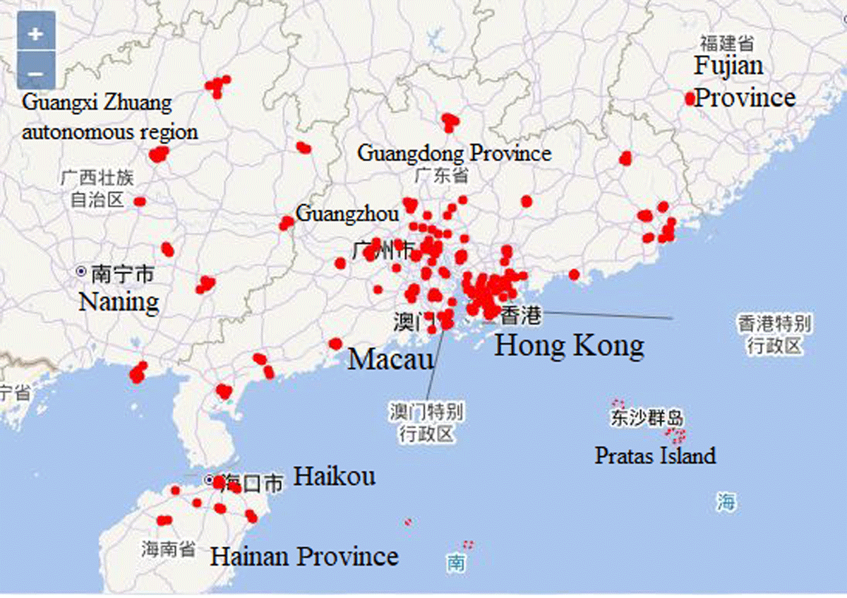
Figure 1
Data sources in southern China including Hong Kong and Macau.
More specifically, the dataset was collected from the Air Quality–China National Environmental Monitoring Center (AQ–CNEMC), the Hong Kong International Airport (AQ–HKIAWEB), the Air Quality Management Information System (AQMIS) and the Macao Meteorological and Geophysical Bureau (AQ–MASMG). The dataset, detailed in Table 2 consists of five pollutants: Respirable Suspended Particulates (RSP), Fine Suspended Particulates (FSP), Nitrogen Dioxide , Ozone and Nitrogen Oxides . The Nitric Oxide (NO) and Nitrogen Oxides ) data was collected from 15 general and 3 roadside stations set up by the Environmental Protection Department (EPD) in different districts of Hong Kong, providing hourly, daily, monthly and annual average concentrations of each pollutant.
Each of the data items , and was sampled from multiple stations. The period discretisation into January, April, July and October, was given by design, reflecting the seasonal periods of winter, spring, summer and autumn. Day discretisation into night, morning, day and evening formed part of our data preparation for modelling. The proportions of missing data for each pollutant were negligible, thus relevant observations could be deleted without affecting the probability or spatial distributions, i.e., the distributions were consistent before and after deletion.
2.2 Modelling Strategy
Our modeling strategy is based on the objectives described in Section 1.3. Exploratory data analysis of the harmonised data provides useful insights into the choice, design and development of relevant modelling approaches to address the research problem. Identifying associations among data attributes like pollutants, timelines and locations, as well as estimating and optimising key air quality parameters across samples highlight the paths towards parameter optimisation and replicability of the chosen methods across the SDG spectrum, which addresses part of our study objectives. Thus, the strategy derives from known theoretical aspects of maximisation and optimisation, which are covered in Sections 2.2.1 through 2.2.3. However, given the random nature of training, validation and testing data, the obvious option is to seek “robust estimates” of relevant parameters, which is what the two algorithms in Section 2.2.4 are designed to deliver.
2.2.1 Computational Maximisation of the Log-Likelihood
Some aspects of data visualisation are presented in Section 3.1 to convert a complex scenario into an easy one, which is useful for readers with limited knowledge of statistics. The popularity of data visualisation across data science applications is well documented (Liang et al., 2023; Pika et al., 2021). However, data visualisation has its limitations, particularly when the interest lies on representing characteristics of high-dimensional data. Under such circumstances, density estimation methods, maximum likelihood and posterior estimations are the most appropriate methods.
It is reasonable to assume that the collated data variables are independent and identically distributed, i.e., they are mutually independent, with the same probability distribution. Let us denote the five pollutants by simple distributions
where represent basic distributions and are group proportions or mixture weights. This implies that we can describe multimodal distributions of any dimension, which we would otherwise only clearly visualise in a 1, 2 or 3-dimensional space. Consider the components of a Gaussian Mixture Model, each with parameters and .
where are the free parameters of the distribution. Let us denote the pollution data in Table 2 by where are independent and identically distributed from some unknown distribution It can be shown that Equation 2 leads to a set of dependent simultaneous equations that can be solved iteratively. To estimate the aggregate distribution representing density distributions such as those exhibited in Figure 5, we can initialise mixture components as follows:
Given the estimated aggregating density in Equation 2 will depend on the weights assigned to each of the components, as defines prior memberships to each–i.e., prior probability of the type of pollution. The maximum likelihood estimate of the free parameters is given as follows:
where each of the likelihood terms is assumed to be a Gaussian Mixture Model density, with the log likelihood
For a single Gaussian model, the sum over vanishes, and Equation 5 reduces to
The parameters that maximise the log likelihood in Equation 5 are obtained by maximising the derivatives of the mean (), variation () and group proportions () with respect to , as follows
Note that the expression in Equation 7, i.e., the necessary conditions for maximising Equation 5, are of the form
where are model parameters, is the probability of data , given hence
The expressions in the denominator in Equation 9 imply that the probability of data given parameters is proportional to the sum of all the components. It can be further shown that
The left-hand side of Equation 10 is a normalised probability vector that represents the probability that the data was generated by the mixture component, which is directly proportional to the likelihood on the right-hand side. Direct maximisation of the likelihood function of data in the form of a random sample is challenging, so the likelihood and parameters in Equations 1 to 10 can only be obtained by iteratively searching for parameters that maximise
2.2.2 Maximum-Likelihood Parameter Estimation and Maximisation Algorithm
If we envision each observation as being characterised by a parametric finite mixture density, we can treat group membership as missing data and use an adapted version of the EM algorithm to estimate and maximise the parameters and Let be initial classes with an unobservable indicator variable
We can then compute class membership as the probability of class given data, as follows
If class membership, central tendency, and variation parameters were observable, they could be estimated as
where is the estimated proportion of data points in class is the mean within that class and is the variation in that category. However, the parameters are not observable, but we can estimate them from data, at each E step
The estimated parameters are then maximised at the step as follows
2.2.3 Extracting Naturally Arising Groups and Components
The estimated and maximised parameters can be used to guide both unsupervised and supervised modelling and in both cases, they potentially help to avoid over-fitting. We adopt PCA and data clustering for dimensionality reduction. The former seeks to transform a number of correlated variables into a smaller number of uncorrelated variables, called principal components, i.e., we can explain the variance-covariance structure of a high dimensional random vector through a few linear combinations of the original component variables. The variables in Table 2 can be formulated in a generic form as in Equation 16, where each extracted component is estimated as a weighted sum of the variables
Here, denotes the number of components and denotes the number of variables. The vectors are chosen such that the following conditions are met.
for
Each of the , maximises the variance and
The covariance
The principal components are extracted from the linear combinations of the original variables that maximise the variance and have zero covariance with the previously extracted components. From a supervised perspective, extracted components can be viewed as new variables and from an unsupervised perspective, they may be viewed as “clusters”.
Cluster analysis is a method for grouping data according to some measures of similarity. If we assume distinct groups in our dataset, each with a specified centroid, then for each of the vectors we can evaluate the distance from to the nearest centroid from the set as
where is an adopted measure of distance, and the clustering objective will then be to minimise the sum of the distances from each of the data points in to the nearest centroid. Optimal partitioning of the dataset requires identification of vectors that solve the continuous optimisation function in Equation 18.
The solution to Equation 18 relates to the partial derivatives in Equations 7 and 8. Minimisation of the distances depends on the initial values in hence if we let be an indicator variable denoting group membership with unknown values, the search for the optimal solution can be through iterative smoothing of the random vector for which we can compute In a labelled data scenario, Equation 18 transforms to the minimisation of Equation 19
where are described by the parameters and are fitted values. Equations 17 to 19 relate to the K–Means clustering algorithm, which searches for clusters in numeric data based on a prespecified number of centroids. The decision on the initial number of centroids ultimately impinges on the detected clusters, and we attempt to address this issue via the two algorithms, below. Addressing spatio-temporal variations in dataset appeals naturally to dealing with randomness in data (Mwitondi and Said, 2013) and adopting interdisciplinary approaches to gain a unified understanding and interpretation of data modelling. In the next exposition, we present two algorithms: EstiMax and the Sample-Measure-Assess (SMA) algorithm (Mwitondi and Zargari, 2018), developed to address variations in data due to inherent randomness.
2.2.4 EstiMax Algorithm
Algorithm 1 below, adapted from a previous similar work (Mwitondi et al., 2018a), is designed to identify naturally arising structures involving the five pollutants in Table 2 and the associated attributes–Times, DayTimes and Period. It searches for smoothing parameters that optimise the densities in Figure 5, while minimising the effect of randomness (Mwitondi, Moustafa and Hadi, 2013).
Algorithm 1
procedure EstiMax
Set Pollutants data
Set as in Equation 11
as in Equation 13
for do
while do
as in Equation 12
s in Equation 13 through 15
end while
end for
end procedure
The EstiMaxi algorithm provides general mechanics for estimating crucial parameters of the pollutants and their likelihoods. Our interest is to obtain multiple sets of parameters in the sampled periods for accurate and consistent estimation. We can then associate the parameters across samples with the time-related variables in Table 2. The SMA algorithm (Mwitondi and Said, 2021) below, invokes the EstiMax, performs comparative analysis and determines the best model. However, this sequential relationship is not a requirement for implementing either of the algorithms, because the EstiMax can estimate parameters from any input dataset, while the SMA can be executed with any predetermined parameters.
The population error will always be greater than or equal to the training sample error drawn from the same population, hence the expected difference is guaranteed to be greater than or equal to 0 (). Section 3 focuses on exploratory data analyses, optimal estimation of the key parameters for the pollutants in Table 2, and their spatio-temporal associations, thus providing insights into assessing pollution patterns and relevant dynamics in southern China. The modelling techniques adopted—PCA, K-Means and the EM algorithm—are based on their underlying mechanics, particularly the influence of the starting point for the last two and their adaptability to the two algorithms.
3 Implementation
Application of the methods to the selected datasets is predicated on the premises that variations in data sources, quality and interpretations entail a good understanding of the overall behaviour of data, as a crucial performance indicator. This section covers exploratory data analysis, identifies naturally arising structures in the sampled data and builds associations among different pollutants over different time periods across the collected samples.
3.1 Exploratory Data Analysis
Exploratory data analysis is a standard method that is usually deployed ahead of data modelling to provide useful insights into understanding data. It delivers key characteristics of targeted datasets, often through numerical and visual summaries (Komorowski et al., 2016). It helps in revealing the overall data behaviour, in detecting patterns, and in spotting anomalies (Ridzuan and Zainon, 2022), as well as being useful in checking the validity of assumptions. Most importantly, its results are useful guidelines to evaluate the appropriateness of modelling techniques.
The left-hand side panel of Figure 2 shows hourly time series of and concentrations, during the investigated time period, measured in micrograms per cubic metre The right-hand side panel are for and measured in “parts per billion” (ppb)–a concentration unit for the number of parts of a substance per billion parts. In both cases, the horizontal axis displays the study period in hours. The time series shows pollution patterns across pollutants. For instance, they generally tend to be lower during the summer period and higher during winter –towards the beginning and end of year. Both and have the highest hourly pollution levels during the first 700 hours of the year and lowest during the last half of the year. Further, pollution appears to be within the same margins throughout the year, whereas tends to peak at regular intervals after the first third of the year. We can relate these patterns to variables of interest such as DayTimes and Period, to assess the time effect of pollutants.
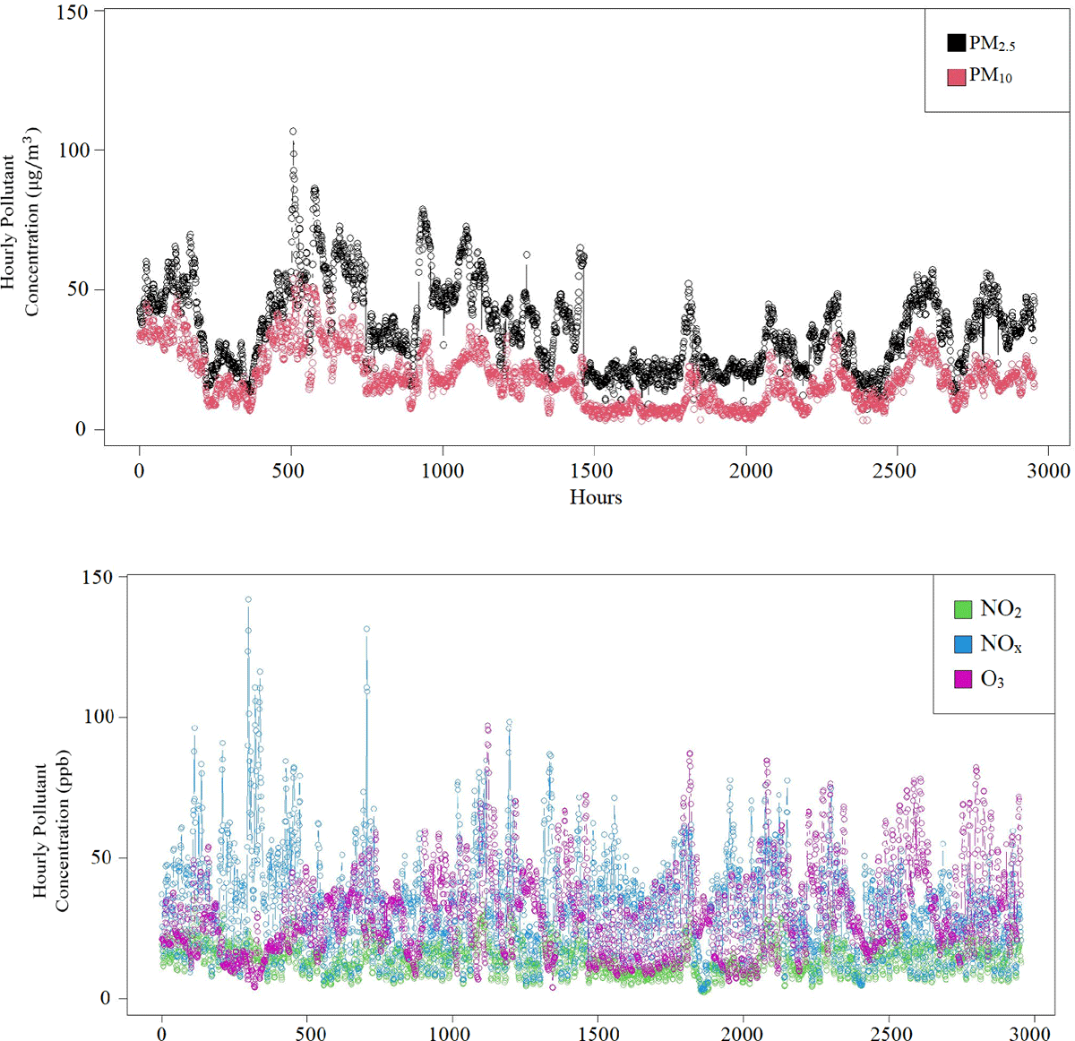
Figure 2
Hourly averaged concentrations for all sampled pollutants.
The time series plots in Figure 2 span across a four month period—January, April, July and October—each further discretised into a repeating sequence of “Night, Morning, Day, Evening” (in Table 3), with corresponding “Start” and “End” hours as shown in Table 2. These trends can also be visualised based on daily averages, in which case patterns representing categories of day, i.e., night, morning, day and evening, can be seen (see Table 4). Steps 8 to 18 of Algorithm # 2 can be applied, with appropriate parameters, to sample through the data for other choices of interest, e.g., day and night or half months. The plots of pollution trends for the four months were fairly consistent with Figure 2.
Table 3
Daily and monthly averages.
| START HOUR | END HOUR | HOURS RANGE | CATEGORIES OF DAY |
|---|---|---|---|
| 00:00hrs -Jan-2023 | 23:00hrs -Jan-2023 | hour | Night, Morning, Day, Evening |
| 00:00hrs -Apr-2023 | 23:00hrs -Apr-2023 | hour | Night, Morning, Day, Evening |
| 00:00hrs -Jul-2023 | 23:00hrs -Jul-2023 | hour | Night, Morning, Day, Evening |
| 00:00hrs -Oct-2023 | 23:00hrs -Oct-2023 | hour | Night, Morning, Day, Evening |
Table 4
Daily and monthly average concentrations of each pollutant.
| AVERAGE TIME | |||||
|---|---|---|---|---|---|
| PERIODS | ppb | ppb | ppb | ||
| Day | 20.08 | 15.77 | 38.00 | 39.51 | 35.52 |
| Evening | 21.51 | 15.99 | 35.85 | 30.29 | 38.41 |
| Morning | 19.96 | 13.61 | 34.79 | 23.70 | 34.68 |
| Night | 19.60 | 11.05 | 22.37 | 25.47 | 35.35 |
| January | 28.36 | 15.30 | 39.38 | 26.06 | 45.01 |
| April | 19.51 | 15.93 | 33.47 | 34.17 | 41.77 |
| July | 9.05 | 11.69 | 35.56 | 29.44 | 23.05 |
| October | 20.14 | 14.49 | 29.79 | 35.79 | 33.84 |
3.2 Understanding Distributional Behaviour
Table 4 exhibits day and annual average pollution levels, where and are lowest in July. The monthly average concentration is 19.26 (with a standard deviation of 7.91 ), and the corresponding daily average is 20.29 (with a standard deviation of 0.84 ). The corresponding monthly and daily averages (deviations) for are 14.35 (1.86) ppb and 14.11 (2.30) ppb respectively. For , the corresponding values are 34.56 (4.00) ppb and 32.75 (7.04) ppb respectively, whereas for and , the corresponding averages and variations are 31.37 (4.44) ppb, 29.74 (7.08) ppb, 35.92 (9.78) ppb and 35.99 (1.65) ppb respectively. The periodic averages in Table 4 and the variations stated above, provide a summary of the pollutants’ distributional behaviour.
Over time, the parameter variations in Table 4 can be used to guide optimisation models for pollution monitoring. Our strategy is to apply algorithms 1 and 2 to estimate, maximise and compare key parameters of pollution. Figure 3 exhibits how central tendency and variation parameters can vary over time. Monthly averages (in red) and standard deviations (in blue) are shown in Figure 3a, while Figure 3b shows the equivalent daily averages.
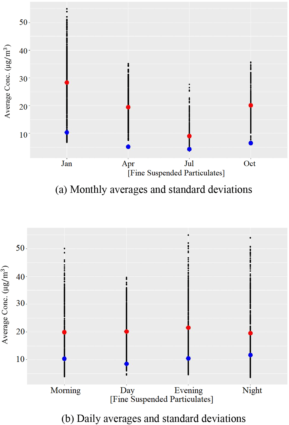
Figure 3
Fine suspended particulates monthly and daily averages and variations.
As an example of the time-related patterns of pollution, consider the distribution of levels over the year, as exhibited in Figure 4. It can be observed that attains its highest concentration during January for all four discretised time periods of day, and that the lowest concentration occurred in July 2023. The variation across different time periods within a day (particularly during July) when pollution levels drop before rising again, is of interest. Understanding the behaviour of such spatio-temporal variations is crucial to gain insights into ways of mitigating the potential impacts of air pollution on the well-being of our surrounding environment and neighbourhoods.
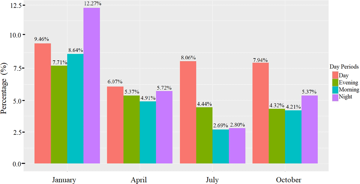
Figure 4
Pollution levels across the year 2023.
Figure 5 shows the density plots for the hourly averages across day time periods, computed across stations, of each of the five pollutants. The horizontal axes in Figure 5a and 5b are micrograms per cubic metre and ppb respectively. In both cases, each density is associated with free parameters that describe its structure, centrality and dispersion, i.e., group membership, mean and variation respectively. These examples are based on datasets acquired from eight stations in southern China: Station-1 (CB_R), Station-2 (CL_R), Station-3 (XCNAQ245), Station-4 (XCNAQ246), Station-5 (XCNAQ250), Station-6 (XCNAQ252), Station-7 (XCNAQ253), and Station-8 (
The sampled stations are distributed in different parts within our investigated domain, thus serve as good representatives of pollution figures across the sampled region. It is important to note that the sensors used for data recording adopt different measurement techniques and therefore the densities in Figure 5 are not intended for direct comparison. However, their variation patterns can be used to gain useful insights into different pollutants on a typical day.
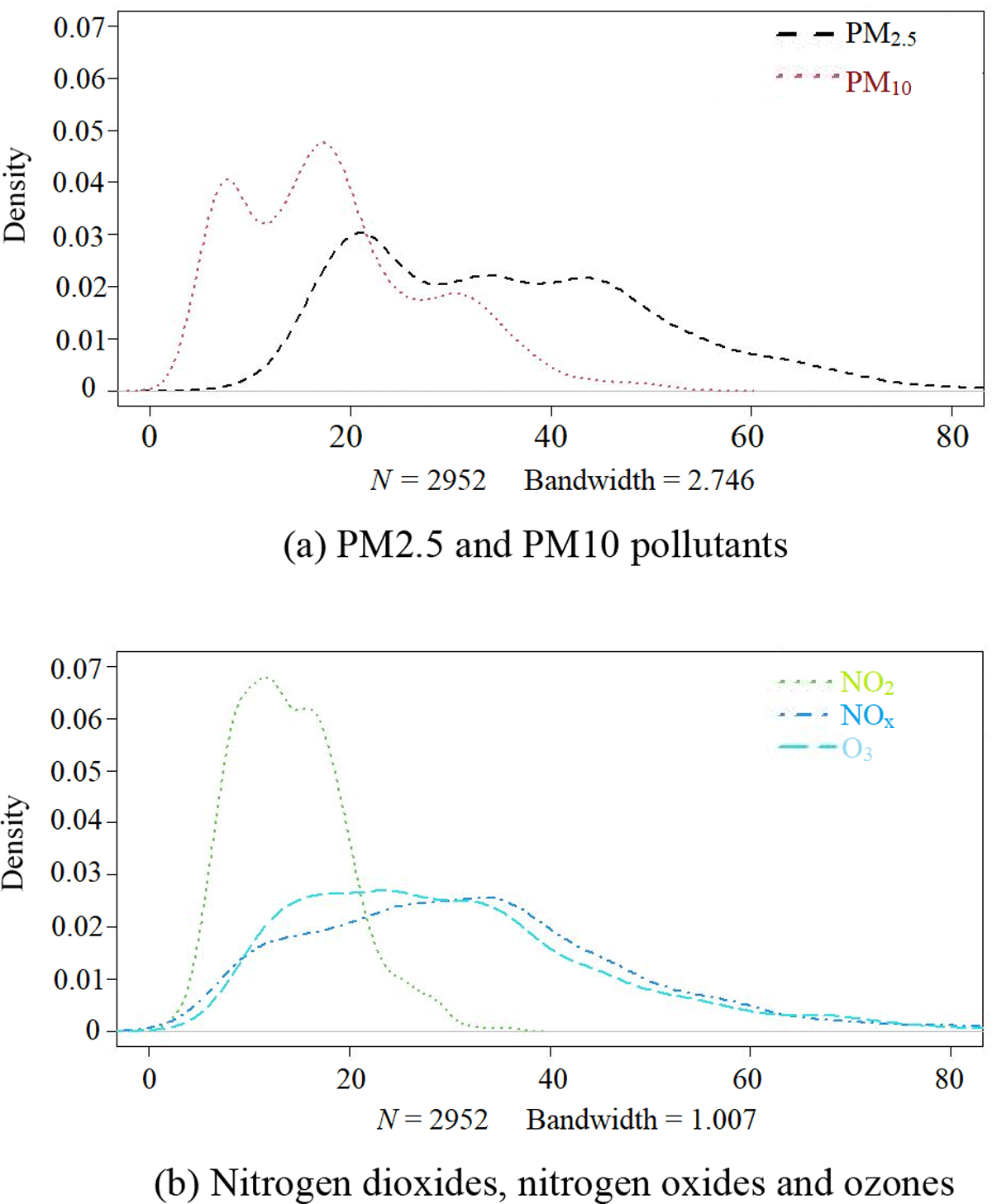
Figure 5
Density distribution of pollutants across day time periods.
3.2.1 Optimisation of Parameters
Figure 6 shows a 2–dimensional clustering of raw pollution datasets, which allows readers to obtain a clear visualisation of the numeric data presented in Table 2. The data points are represented by points in the ellipsoid plots, using principal components or multidimensional scaling. We use the method to illustrate the optimisation process adopted in estimating , as defined in Equation 2. The plots represent a set of two, three and four clusters generated from average pollution levels of the five pollutants. Each of the three set of clusters is formed around a set of centroids that can be determined in a number of ways–such as random initialisation or data–dependent parameters.
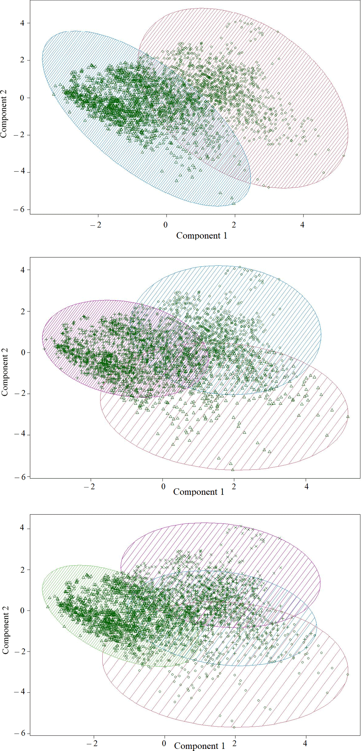
Figure 6
Pollution data points on a multidimensional scaling.
Table 5 exhibits the contributions of each pollutant into the formation of components, as well as the final centroids for each of the three sets of clusters. In all three cases, the two components contributed 76.41% of the statistical variation.
Table 5
Centroids of the selected clusters formed.
| POLLUTANT | 2 CLUSTER CENTRES | 3 CLUSTER CENTRES | 4 CLUSTER CENTRES |
|---|---|---|---|
| Fine Suspended Particulates () |
|
|
|
| Nitrogen Dioxide (NO_2) |
|
|
|
| Ozones (O_3) |
|
|
|
| Nitrogen Oxides () |
|
|
|
| Respirable Suspended Particulates () |
|
|
|
An illustration of estimation and maximisation of key parameters of the pollutants using the EstiMax algorithm is given in Figure 7a and 7b based on raw and concentrations from the 8 stations in southern China. In each case, the dotted thin lines represent the average across samples and the thick line is the maximised estimated average across the samples. The algorithm does quite well in capturing the multi-modality of the pollutants.
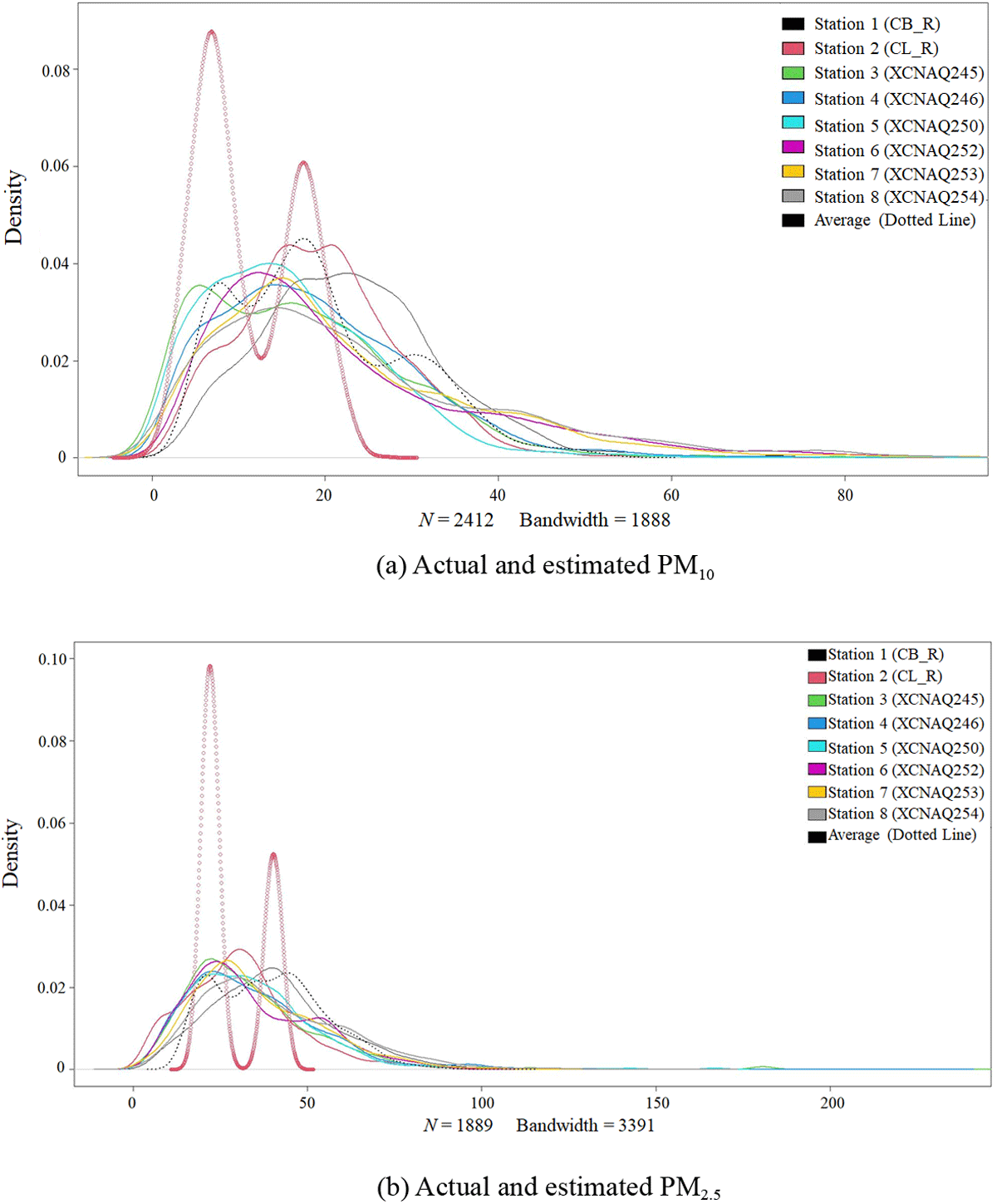
Figure 7
Actual and estimated (Left) and (Right).
The bimodality of the estimated pollution levels across the eight stations were the best results after comparing 2, 3, 4 and 5 modes, in relation to the raw patterns. The bimodality, effectively, implies that there are two pollution levels across the eight monitoring stations: high and low, although there are clear outliers in the upper tails in each case.
3.2.2 Extracting Components
If we denote the overall state of pollution by , our interest lies on the multicollinearity of the known factors, which cause inaccurate estimates of various parameters, and as a result affect future modelled outputs or forecasts. One way of addressing this issue is to apply PCA –a statistical method that reduces data dimension, and maximises variation within the same dataset. Ultimately, this results in the estimation of parameters in Algorithm 1, which improves the accuracy of for being used as prior information for ongoing pollution monitoring within a prescribed spatial domain.
Figure 8a shows the correlation figures among each pair of the five pollutant variables, while Figure 8b shows the extracted components. In this case, the standard deviations in Component 1 through Component 5 are 19.26, 17.18, 13.24, 4.46 and 3.01, with proportions of variance equal to 0.426, 0.339, 0.201, 0.0228 and 0.010 respectively. Note that the first two components account for 76.5% of the variation in the pollution dataset.
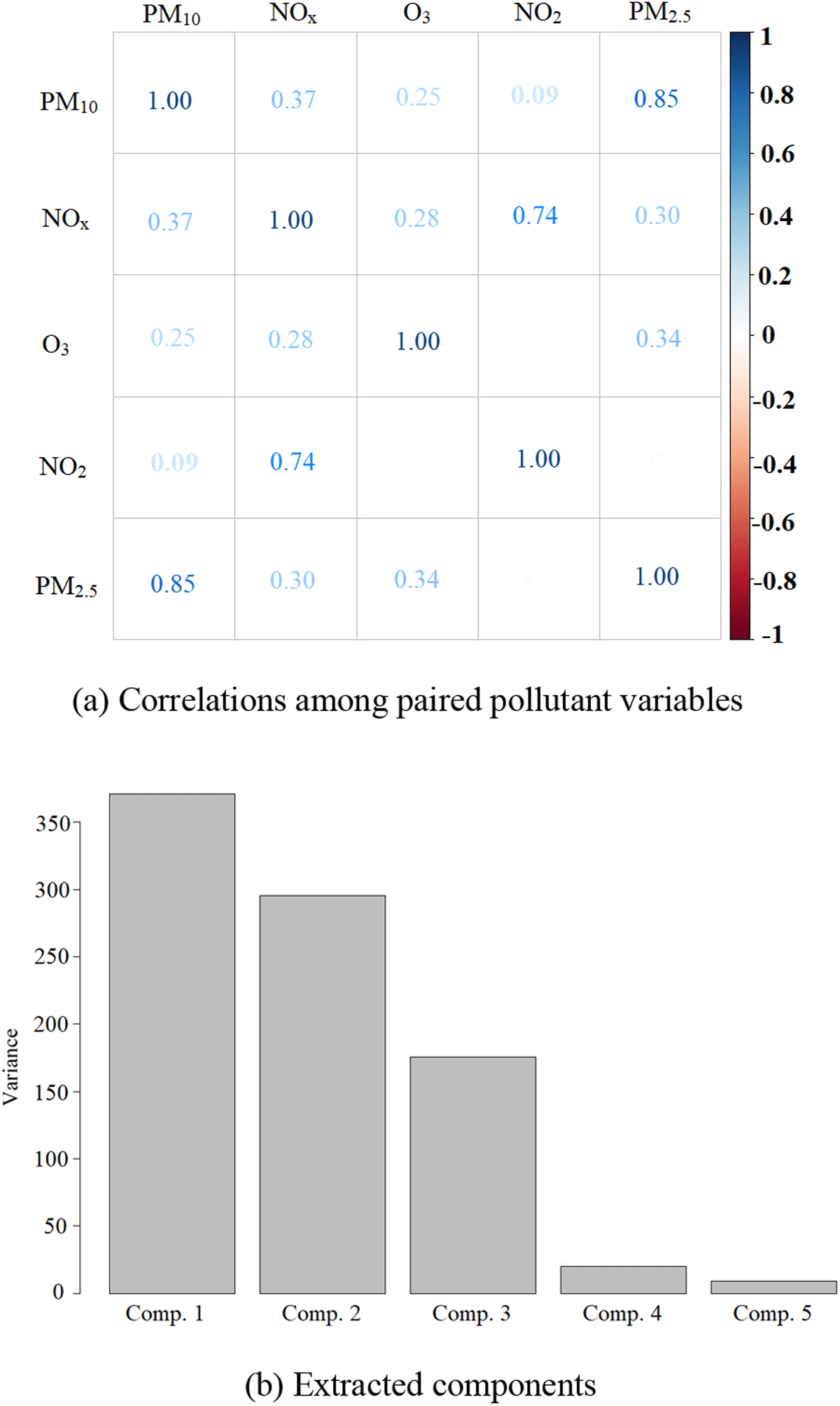
Figure 8
Correlations among paired pollutant variables.
Table 6 shows the contribution of variables in each component. It can be seen that has a very strong relationship with component 4, while the absence of Nitrogen Oxide in Component 2 is most pronounced, as is that of Nitrogen Dioxide in Component 5. Similarly, the absence of ozones in Component 3 is seemingly vital in its formation.
For a clearer interpretation of the numerical and graphical results in Section 3, we need to relate them to the modelling strategy in Section 2.2–particularly to Algorithms 1 and 2. Part of the modelling strategy provides the theoretical foundations on which we can understand the overall data behaviour, and part of it provides aspects of its practical implementation. The main idea is to attain optimal interpretability of modelling results which, typically, derive from training and validating statistical models on “random samples” and ultimately applying them on new data that is also “random”, entailing variations across samples. Note that, mathematically, from an dimensional dataset, a total of components can be extracted, but, usually only a few will explain the variation in the data. It is the foregoing data variation that Algorithms 1 and 2 seek to address. For instance, the centroids of the formed clusters in Table 6 are based on 1, 2, 3, 4 and 5 clusters, although for PM10 and Ozone, the maximum of 75 and 114 respectively could have been extracted. Drawing new samples of PM10 and Ozone from similar data sources isn’t necessarily going to generate the same number of components or the same loadings. The five clusters in Table 6 are judged optimal according to the repeated sampling via Algorithms 1 and 2. The same applies to correspondence analysis.
3.2.3 Correspondence Analysis
The average pollution levels for each of the five pollutants from each of the eight locations are given as continuous data. Their density plots exhibit multi-modality –a distributional behaviour that is supportive of discretisation of each variable. If we denote the average vector by we can discretise it by setting the following rule:
Equation 20 describes how an ordered continuous data vector can be visualised based on its overall behaviour. Mean estimates are in accordance with the EstiMax algorithm, and initial points can range from completely random to data-dependent, such as those in Figure 3 or other data parameters, such as using percentiles or quartiles. In each case, a quantitative vector is broken down into discrete segments that form categories of visual analysis based on correspondence analysis. The technique enables the visualisation of associations between different categories of selected data attributes in a 2–dimensional space. It seeks to establish associations between some row elements and some column elements, generating orthogonal components, with maximisation of variation in the data in mind.
Figure 9a represents associations between discretised averages with the Time of Day, while Figure 9b shows the same association with annual periods. In both cases, the axes measure the levels of variation in the data, with the extreme left of the horizontal axis representing the negative measure and the extreme right representing the most positive measure. Similar definitions are applicable for the south and north directions of the vertical axis. The highest variation in both panels is accounted for by the first component, at 95.7% and 92.7% respectively.
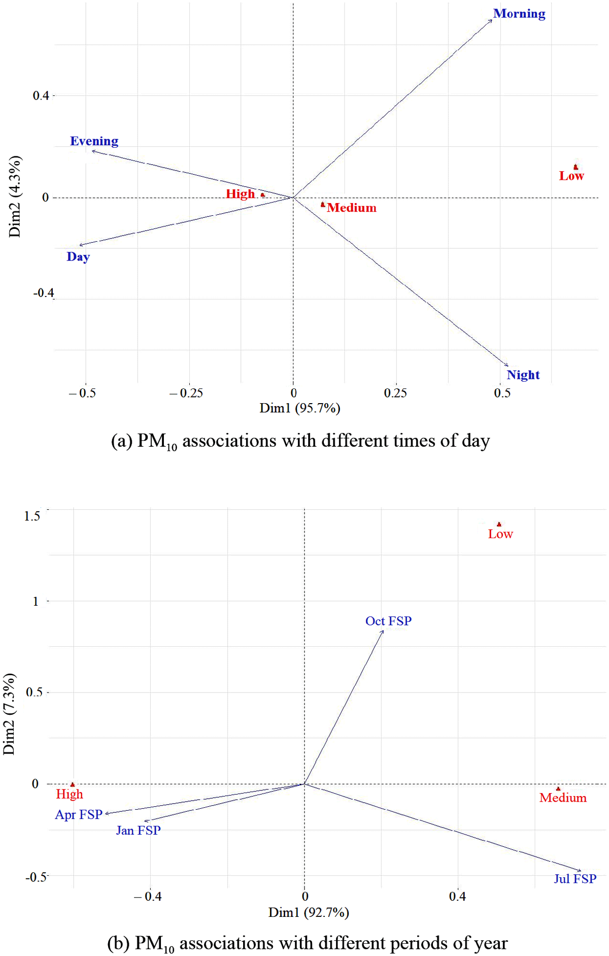
Figure 9
associations with daily and annual periods.
Tables 7 and 8 represent the frequencies of each of the three categories during the day and the year 2023, respectively. Note how the High and Medium categories dominate in each case. It is worth mentioning that this distribution is, and should always be, conditional on the distributional behaviour of the discretised variable, since the number of classes does affect how many cases fall into each class. Our interest in Figure 9 is to find out the points that contribute to the solution provided by the method which, in this case, presents associations between the pollutants and with different time periods. CA forms these patterns based on “expected values”–associating row and column labels for the disparity between “expected” and “observed” values, in order to explain the percentage of variance in the data.
Table 7
Row points vs Principal Dimension 1.
| HIGH | LOW | MEDIUM | |
|---|---|---|---|
| Day | 484 | 4 | 373 |
| Evening | 352 | 3 | 260 |
| Morning | 369 | 20 | 349 |
| Night | 351 | 17 | 370 |
Table 8
Columns vs Principal Dimension 1.
| HIGH | LOW | MEDIUM | |
|---|---|---|---|
| January | 587 | 0 | 157 |
| April | 618 | 0 | 102 |
| July | 58 | 4 | 682 |
| October | 293 | 40 | 411 |
Figure 9a shows the relationship between and times of day. The strength of the relationship is measured by the distance between two points and the tightness of the angle: the tighter the angle, the stronger the relationship, e.g., the angles formed between “Day” and “Evening” with “High” pollution. Orthogonal angles () indicate no relationship, while a angle indicates negative association. The length of the line connecting the row label to the origin indicates the strength of the row label association, e.g., “Morning” and “Night” with respect to “Medium” and “Low” pollution levels. Being farther away from the origin means more closely associated with the factors in the proximity. In Figure 9a and 9b, most time periods are farther from the origin, without being very close to any factor.
Table 9 presents the row points, most associated with the first principal dimensions (PD) for the association between and Day Times, while Table 10 presents similar information for with annual periods. Evening times and January have the lowest row points association with the second PD, whereas Night Times and October have the highest association with the second dimension. These are quite interesting patterns, worth following through as they potentially indicate commonalities between those periods which may relate to specific activities or lack of them.
Table 9
Row points vs PD 1 for Day Times.
| DIMENSION 1 | DIMENSION 2 | |
|---|---|---|
| Day | 26.50596 | 3.576712 |
| Evening | 23.52921 | 3.377988 |
| Morning | 23.04545 | 49.011043 |
| Night | 26.91938 | 44.034257 |
Table 10
Columns vs PD 1 for Annual Periods.
| DIMENSION 1 | DIMENSION 2 | |
|---|---|---|
| April | 26.778387 | 2.672733 |
| January | 17.240575 | 4.196079 |
| July | 51.795246 | 22.524998 |
| October | 4.185793 | 70.606190 |
A further comparative analysis from eight different stations is provided in Figure 10, in which and are compared for stations 1 and 8, positioned further apart from each other. The top two panels present concentrations, while the bottom panel presents concentrations within the same stations. In both cases, variations within the four months of 2023 are more obvious than variations within different periods of a day.
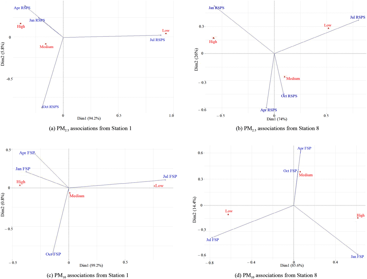
Figure 10
and associations from Stations 1 and 8.
The discretisation in Equation 20 provides the comparative basis in line 15 of the SMA algorithm (Algorithm 2), which can be visualised via plotting. On the basis of such comparison, one can update parameters within the algorithm, and conduct corresponding assessment of to determine the difference between predicted and actual parameters.
Algorithm 2
procedure SMA
Set Pollutant datasets
Set initial clusters
Call Algorithm 1
Comparative parameters
Learn based on a chosen learning model
for do: Set large and search for optimal values iteratively
while do Vary sample sizes to up to the nearest integer 50% of
with current parameters
Using visual plots and/or animation
end while
end for
based on
end procedure
4 Concluding Remarks
This paper proposed a data-driven robust method for addressing societal challenges, focusing on air pollution –a problem that cuts across disciplines, sectors and geographic borders. The focus on air pollution, SDGs and southern China was inspired by the human–nature interactions and their mutual impact, as we know them, i.e., air pollution affecting and/or being affected by different SDGs. The link between air pollution and various aspects of SDGs, the need for developing a replicable model and the choice of the study area were used to highlight the purpose of the study. Focusing on southern China was motivated by the country’s global role as a polluter and mitigator of pollution, while the focus on “robustness” was motivated by the need for developing models that could be replicated in a spatio-temporal context. The main idea was to use the “most parsimonious model” to highlight potential data–driven solutions to more complex regional and global scenarios. It was assumed that gaining insights into spatio-temporal patterns of the common pollutants in southern China would highlight the path towards mitigating the impact of pollution elsewhere. It was further assumed that the overall pollution levels in southern China were mainly contributed by the five major pollutants within the region, and that these five attributes could be used as predictors of the pollution levels in the region and, potentially, elsewhere.
The paper investigated associations among common air pollutants in southern China during specific months in 2023 and at different times of a day. Its key motivation was twofold. Firstly, human and natural activities constantly generate multifaceted pollution data much faster than our ability to process them and, secondly, most environmental modelling approaches still face model optimisation challenges that derive from inherent randomness in data (Mwitondi, Munyakazi and Gatsheni, 2018b). Hence, developing tools and methods for harnessing, processing and sharing such data is crucial to address a wide range of societal challenges, such as human health, food security and other SDG-related challenges and opportunities.
Two algorithms were used to maximise and optimise air quality parameters that best describe associations between different attributes of interest, e.g., between specific pollutants and timelines; they provided insights into policy formulation on spatio-temporal mitigation of air pollution. They also generated static, interactive and easily interpretable visual outputs, that are pivotal in optimising operational efficiency. For instance, the parameters in Figure 3 relate to monthly and daily averaged concentration figures, which are subject to spatio-temporal variation. Monitoring such variation within and across samples is crucial to improve our understanding of how a specific spatial domain could be affected by pollution that occurs in the lower atmosphere. Further, the algorithms used unobservable (latent) variables to reduce data dimensionality, and combined observable variables to make them more interpretable. While the algorithms balance the power of data, machine learning techniques and underlying domain knowledge, they also contribute towards attaining mutual understanding across fields and sectors. Overall, the current study has implemented rigorous interdisciplinary approaches in combining sophisticated data science algorithms and relevant domain knowledge of our atmosphere.
A comparative analysis with previous studies was based on model optimisation, which is what the two algorithms sought to achieve. The novelty of the study hinges on addressing data randomness and on highlighting the path to addressing the ‘non-orthogonality’ of SDGs. The two algorithms were used to generate optimal associations of temporal patterns (within different hours of the same day, monthly or annually) with relevant pollutant attributes; they provided particularly useful insights into our understanding of the overall state of pollution within the atmosphere of the southern China region, Hong Kong and Macau. Balancing the power of data, machine learning techniques and underlying domain knowledge through the two algorithms exhibited superiority over standard machine learning applications. Identifying such associations aligns with the key aspects of SDGs, particularly their “non-orthogonality”, and it can help to highlight paths to a unified and interdisciplinary understanding of the triggers of the SDG indicators.
The two general and seven specific objectives in Section 1.3 were fully met, except objective #2 (b), which remains a subject for further research. However, the findings of this research will contribute to a better understanding of how to deal with the challenges posed by the non-orthogonality of socioeconomic, technical, and environmental attributes of the SDGs. That is because the non-orthogonality of SDGs masks a lot of potentially useful data that researchers need to dig up and share publicly with the wider scientific community, as well as with policymakers. For that, there is no better testing ground on how to build analytical bridges across disciplines and sectors than on the SDG spectrum. This work is expected to highlight novel directions into the environmental and other aspects of SDG modeling. It is worth noting that applications of the proposed techniques are not confined to air pollution. The two algorithms are readily adaptable to anomaly detection for use in different applications in industry, medicine and business (Li and Jung, 2023; Li et al., 2023). In this application, however, rather than just uncovering “abnormal” events, we mapped them to periodic patterns and, hence, provided better insights to stakeholders, which potentially connects to and influences policymakers.
Acknowledgements
We would like to thank our respective institutions – Qatar University, SESRI Institute; The Chinese University of Hong Kong, Department of Mathematics; and The Hong Kong University of Science and Technology, Department of Mathematics, for allowing us time to complete this manuscript. We are also deeply grateful to all those who reviewed the manuscript at different stages of its development, and who provided very constructive suggestions, most of which we adopted. Last, but not least, this work would not have been completed without the patience and support of many colleagues, friends and family members whose daily lives were touched by the development of this work.
Competing Interests
The authors have no competing interests to declare.