
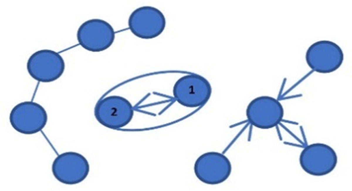
Figure 1
Reciprocal nearest neighbor relationship between datapoint 1 and datapoint 2.
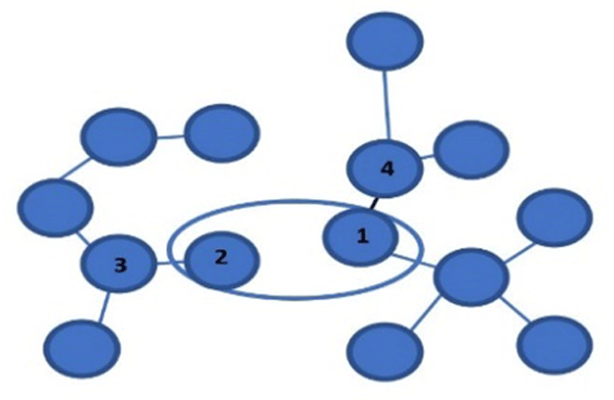
Figure 2
Formation of isolated subgroups within a cluster due to neighbor relations.
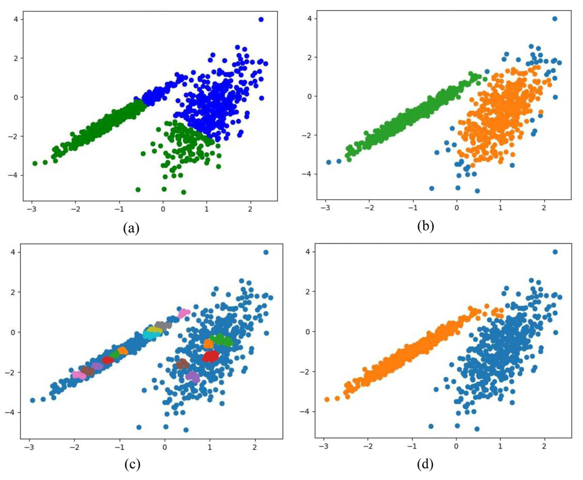
Figure 3
Comparison of clustering algorithms on 2D-synthetic data sets with two clusters (a) K-means clustering results, (b) DBSCAN clustering results, (c) OPTICS clustering results, and (d) Birch clustering results.
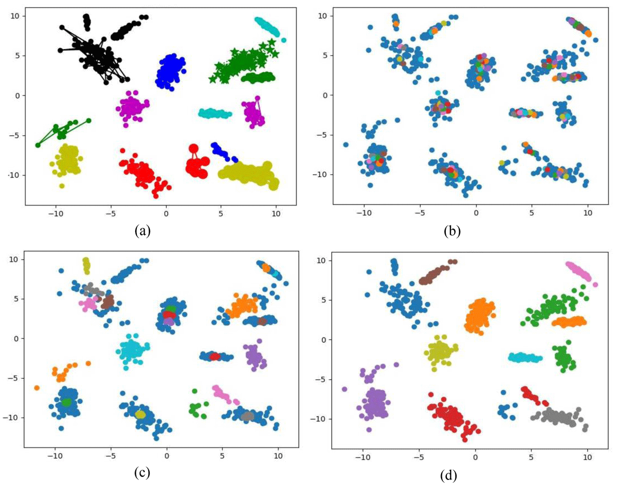
Figure 4
Comparison of clustering algorithms on 2D- synthetic data sets with 15 clusters (a) K-means clustering results, (b) DBSCAN clustering results, (c) OPTICS clustering results, and (d) Birch clustering results.
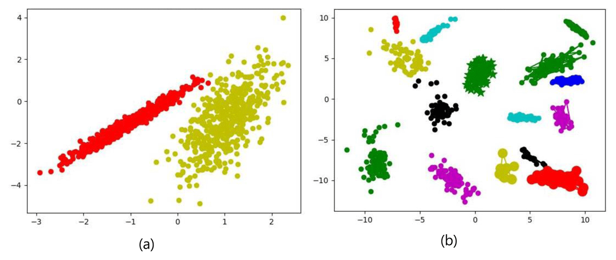
Figure 5
Performance comparison of BHC-Clustering against other algorithms.
Table 1
Characteristics of real-world datasets.
| DATASET (DS) | NUMBER OF INSTANCES | CLASSES | DIMENSION |
|---|---|---|---|
| Iris Plants | 150 | 3 | 4 |
| Wine | 178 | 3 | 13 |
| Breast Cancer (BC) | 569 | 2 | 30 |
| Seeds-Dataset (SD) | 210 | 3 | 7 |
| Glass Identification (GI) | 214 | 6 | 9 |
Table 2
Predicted and actual number of classes and accuracy rates of clustering algorithms on real-world datasets.
| DS | # OF CLASSES | ACCURACY % | ||||
|---|---|---|---|---|---|---|
| PRED. | ACT. | BHC-CLUST. | DBSCAN | OPTICS | K-MEANS | |
| Iris | 3 | 3 | 90.7 | 66 | 67 | 24 |
| Wine | 3 | 3 | 62 | 33 | 67 | 16 |
| BC | 2 | 2 | 70.3 | 63 | 72 | 85 |
| SD | 3 | 3 | 63 | 28 | 18 | 26 |
| GI | 6 | 6 | 76.2 | 23.8 | 16 | 45 |
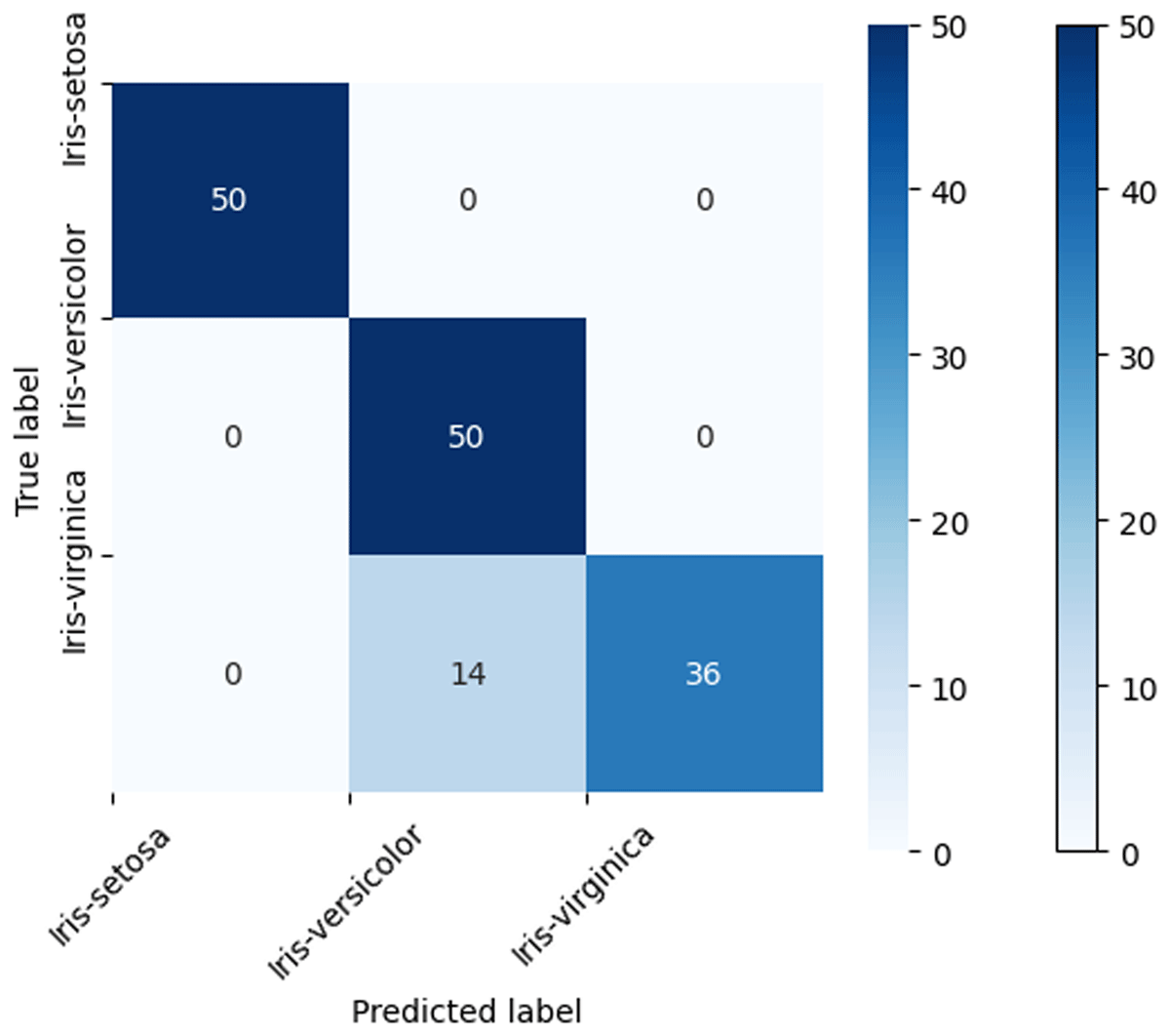
Figure 6
Confusion matrix for Iris dataset clustering using BHC algorithm.