
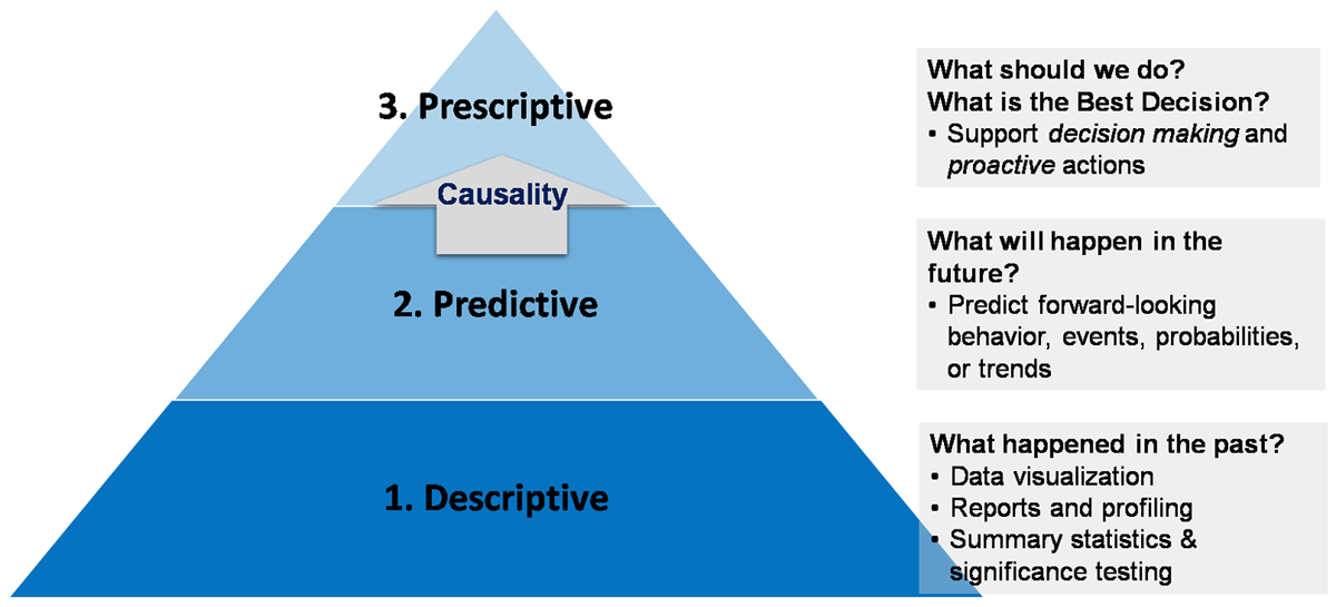
Figure 1
Three types of analytics (Lo 2020).
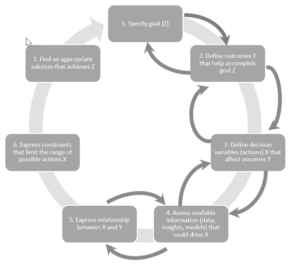
Figure 2
Proposed causal prescriptive analytics framework.
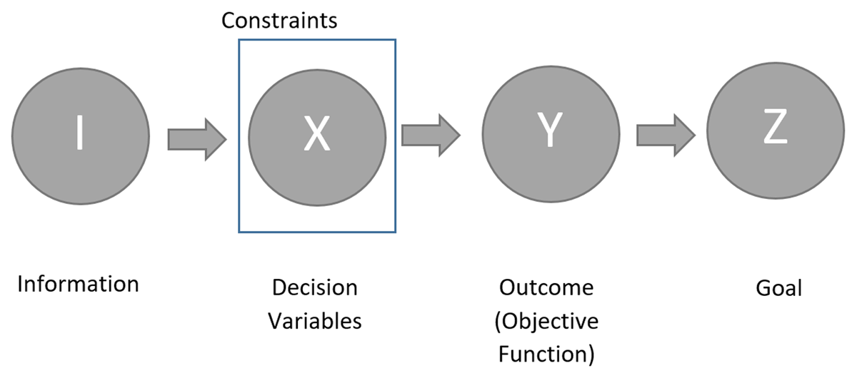
Figure 3
Directed acyclic graph (DAG) representation of the proposed causal prescriptive analytics framework.
Table 1
Examples of problems where the causal prescriptive analytics framework can be applied.
| PANEL A: CAUSAL INFERENCE NOT REQUIRED | ||||
|---|---|---|---|---|
| PROBLEM | DECISION, X | COEFFICIENT, C | IMMEDIATE OUTCOME, Y | ULTIMATE OBJECTIVE, Z |
| Vehicle routing | Selection of arcs | Arc distance | Total travel distance | Travel distance or cost, to be minimized |
| Workforce scheduling | Assignment of employees to shifts | Staffing cost per employee | Total cost | = Y, to be minimized |
| Inventory management | Quantity of raw materials ordered at each time | Holding cost per unit and cost per order | Ordering cost and holding cost | Total cost, to be minimized |
| Portfolio construction | % allocation to each stock | Individual stock returns | Monthly portfolio return | Long-term return, to be maximized |
| PANEL B: CAUSAL INFERENCE REQUIRED | ||||
| Direct marketing (see Appendix A for details) | Assignment of treatment to each customer | Lift in purchase probability due to direct marketing | Incremental sales due to direct marketing | Incremental profit due to direct marketing, to be maximized |
| Pricing | What price to set | Sales volume | Sales revenue | Profit = sales revenue – variable cost, to be maximized |
| Customer retention | Attempt to retain which customer | Change in retention rate due to retention program | Retained or not | Profit = predicted revenue from future sales *P(retention) – cost of retention, to be maximized |
| Employee acquisition | Number of sales agents to recruit | Total sales volume | Total sales revenue | Profit = estimated sales revenue (Y) – cost of total employment, to be maximized |
| Digital health | Message to show to each individual | Message-specific health outcome | Individual health outcome | Employer-level health cost, to be minimized |
| Personalized medicine | Who to receive treatment | Treatment effectiveness | Individual health outcome | Population health, to be maximized |
| Health care policy | Introduce the policy or not | Population readmission rate | Population readmission rate | Health care cost, to be minimized |
| Economic policy | Interest rate level | Consumer and business responses | Consumer and business responses | Overall economic measure, to be improved |
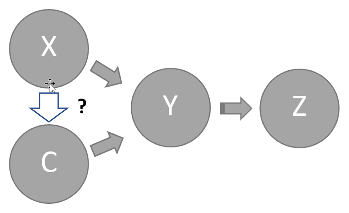
Figure 4
Causal inference in prescriptive analytics problem formulations.
Table A.1a
Optimization using traditional response modeling.
| CLUSTER | CLUSTER SIZE (IN NEW DATA) | MEN’S MERCHANDISE TREATMENT RESPONSE RATE | WOMENS MERCHANDISE TREATMENT RESPONSE RATE | CONTROL RESPONSE RATE | MEN S MERCHANDISE LIFT IN RESPONSE | WOMEN’S MERCHANDISE LIFT IN RESPONSE | DECISION VAR (TREATMENT QUANTITY) ON MEN’S | DECISION VAR (TREATMENT QUANTITY) ON WOMEN’S | TOTAL TREATMENT QUANTITY BY CLUSTER | |
|---|---|---|---|---|---|---|---|---|---|---|
| 1 | 3180 | 0.2549 | 0.2385 | 0.2617 | –0.0068 | –0.0232 | 3,180 | – | 3,180 | |
| 2 | 40 | 0.1779 | 0.1477 | 0.1039 | 0.0741 | 0.0439 | – | – | – | |
| 3 | 9110 | 0.3133 | 0.2425 | 0.1837 | 0.1296 | 0.0589 | 9,110 | – | 9,110 | |
| 4 | 1090 | 0.5385 | 0.2273 | 0.2051 | 0.3333 | 0.0221 | 1,090 | – | 1,090 | |
| 5 | 51300 | 0.1080 | 0.0793 | 0.0451 | 0.0628 | 0.0347 | – | – | – | |
| 5 | 27950 | 0.2106 | 0.1588 | 0.1315 | 0.0791 | 0.0273 | – | – | – | |
| 7 | 67170 | 0.1620 | 0.1440 | 0.0948 | 0.0672 | 0.0492 | – | – | – | |
| S | 4220 | 0.3704 | 0.2817 | 0.2345 | 0.1359 | 0.0472 | 4,220 | – | 4,220 | |
| 9 | 257590 | 0.2218 | 0.2116 | 0.1393 | 0.0826 | 0.0724 | 42,400 | – | – | |
| Total | obj value | 5,597 | – | 5,597 |
Table A.1b
Optimization using uplift modeling.
| CLUSTER | CLUSTER SIZE (IN NEW DATA) | MEN’S MERCHANDISE TREATMENT RESPONSE RATE | WOMENS MERCHANDISE TREATMENT RESPONSE RATE | CONTROL RESPONSE RATE | MEN S MERCHANDISE LIFT IN RESPONSE | WOMEN’S MERCHANDISE LIFT IN RESPONSE | DECISION VAR (TREATMENT QUANTITY) ON MEN’S | DECISION VAR (TREATMENT QUANTITY) ON WOMEN’S | TOTAL TREATMENT QUAITITY BY CLUSTER | |
|---|---|---|---|---|---|---|---|---|---|---|
| 1 | 4,180 | 0.2333 | 0.0970 | 0.0746 | 0.1587 | 0.0224 | 4,180 | – | 4,180 | |
| 2 | 5,650 | 0.2275 | 0.1568 | 0.1623 | 0.0652 | –0.0055 | – | – | – | |
| 3 | 60,220 | 0.1697 | 0.1668 | 0.1040 | 0.0658 | 0.0628 | 2,340 | – | 2,340 | |
| 4 | 12,370 | 0.2854 | 0.2181 | 0.1563 | 0.1290 | 0.0618 | 12,370 | – | 12,370 | |
| 5 | 8,940 | 0.1133 | 0.1221 | 0.0461 | 0.0672 | 0.0760 | – | 8,940 | 8,940 | |
| 5 | 29,240 | 0.1626 | 0.1320 | 0.1107 | 0.0519 | 0.0213 | – | – | – | |
| 7 | 28,070 | 0.2090 | 0.1475 | 0.1222 | 0.0868 | 0.0254 | 28,070 | – | 28,070 | |
| S | 4,100 | 0.4194 | 0.2183 | 0.1944 | 0.2249 | 0.0239 | 4,100 | – | 4,100 | |
| 9 | 37,060 | 0.1216 | 0.1071 | 0.0645 | 0.0572 | 0.0426 | – | – | – | |
| Total | 189,850 | obj value | 5,773 | 680 | 6.453 | |||||