
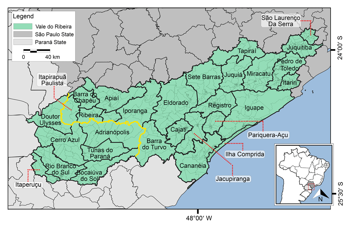
Figure 1
The 30 municipalities of the Vale do Ribeira in southeastern Brazil. The boundary between the States within which the Vale do Ribeira lies is shown by a yellow line. Smaller divisions within each municipality are ‘census sectors’, each containing about 300 households. These census sectors are the finest subdivision available in IBGE publications (https://ibge.gov.br).
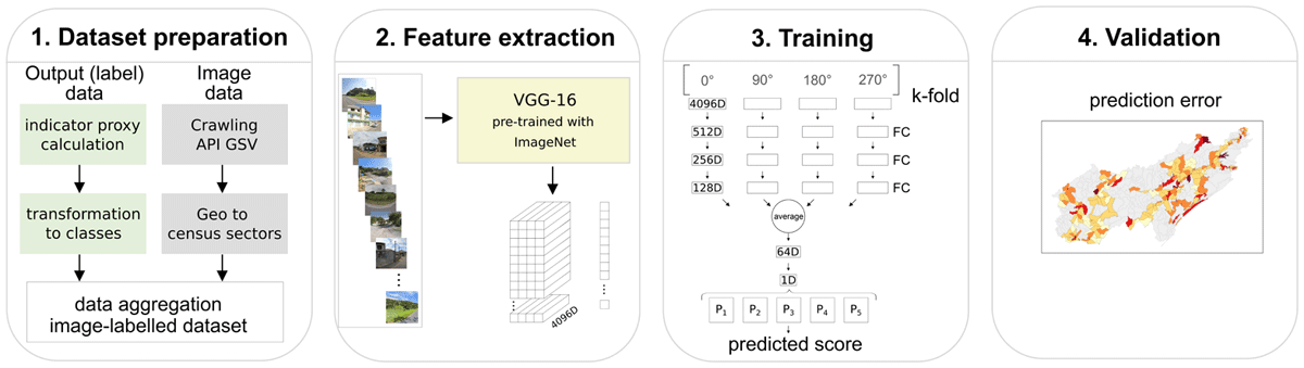
Figure 2
Workflow diagram showing the four main steps: 1) dataset preparation, 2) feature extraction, 3) training, and 4) validation. Street image samples were obtained from Google Street View.
Table 1
Statistics of census sectors, municipalities and states in the Vale do Ribeira.
| STATE | MUNICIPALITY | NUM. CENSUS SECTORS | STATE | MUNICIPALITY | NUM. CENSUS SECTORS |
|---|---|---|---|---|---|
| PR | Adrianópolis | 21 | SP | Itariri | 61 |
| SP | Apiaí | 55 | SP | Itaóca | 9 |
| SP | Barra Do Chapéu | 11 | SP | Jacupiranga | 26 |
| SP | Barra Do Turvo | 14 | SP | Juquitiba | 54 |
| PR | Bocaiúva Do Sul | 23 | SP | Juquiá | 36 |
| SP | Cajati | 38 | SP | Miracatu | 48 |
| SP | Cananéia | 27 | SP | Pariquera-açu | 27 |
| PR | Cerro Azul | 42 | SP | Pedro De Toledo | 17 |
| PR | Doutor Ulysses | 13 | SP | Registro | 69 |
| SP | Eldorado | 30 | SP | Ribeira | 8 |
| SP | Iguape | 60 | PR | Rio Branco Do Sul | 58 |
| SP | Ilha Comprida | 28 | SP | Sete Barras | 26 |
| SP | Iporanga | 19 | SP | São Lourenço Da Serra | 27 |
| PR | Itaperuçu | 34 | SP | Tapiraí | 15 |
| SP | Itapirapuã Paulista | 9 | PR | Tunas Do Paraná | 12 |
Table 2
The Income Score and income range for each HDI income class calculated on a monthly basis. The details of the source data are found in section 6.
| INCOME SCORE | HDI–INCOME VALUE | ABSOLUTE INCOME REFERENCE | USD (2021 6 APRIL) |
|---|---|---|---|
| 1 | HDI [0.00–0.20] | R$ 8.00–R$ 813.00 | $1.41–$143.52 |
| 2 | HDI [0.20–0.40] | R$ 813.00–R$ 1618.00 | $ 143.52–$285.63 |
| 3 | HDI [0.40–0.60] | R$ 1618.00–R$ 2423.00 | $ 285.63–$427.74 |
| 4 | HDI [0.60–0.80] | R$ 2423.00–R$ 3228.00 | $ 427.74–$569.85 |
| 5 | HDI [0.80–1.00] | R$ 3228.00–R$ 4033.00 | $569.85–$711.97 |
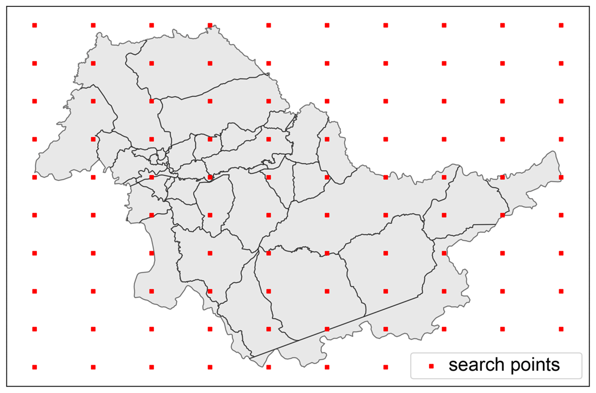
Figure 3
The sampling regime using an example of the Juquitiba municipality. The red dots represent the defined geolocated points searched by the crawler algorithm.
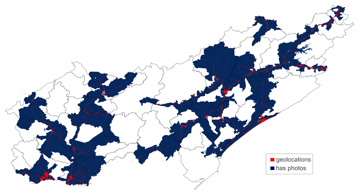
Figure 4
Geolocations at which GSV images were available, the census sectors shown in blue. In white the sectors in which there was no GSV available.
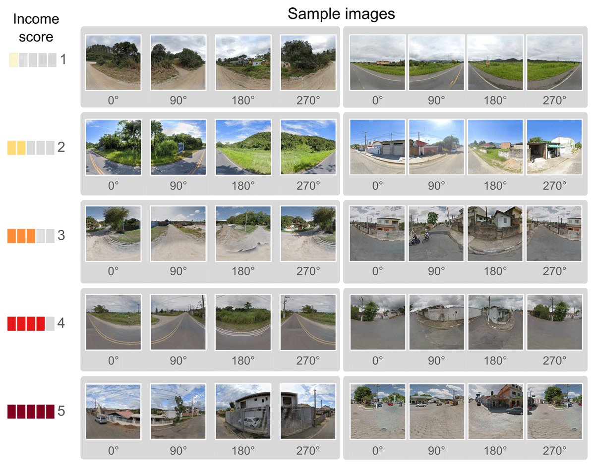
Figure 5
Examples of two panoramic images for each income score taken randomly from Vale do Ribeira. Each image sample was taken over four angles.
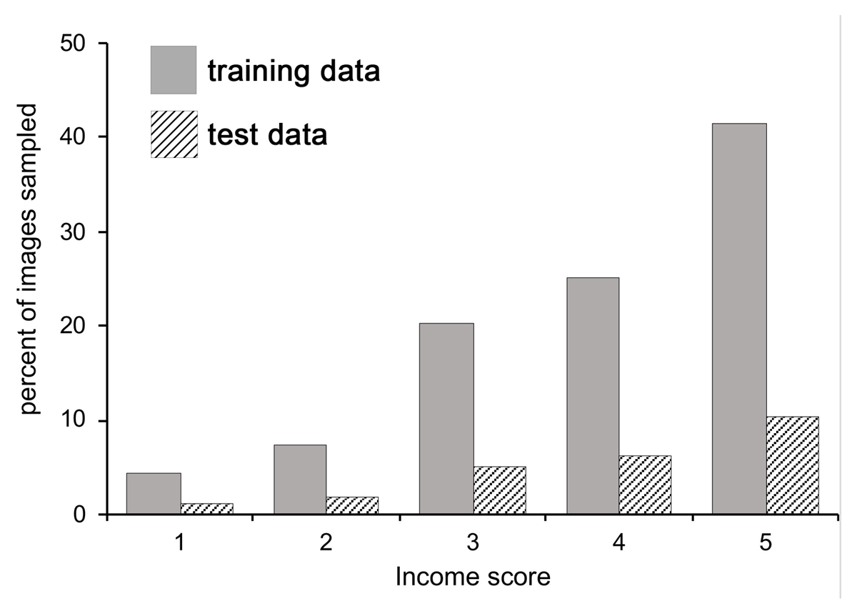
Figure 6
The distribution of images sampled (112,368 in total) for each income score for both the training and the testing datasets.
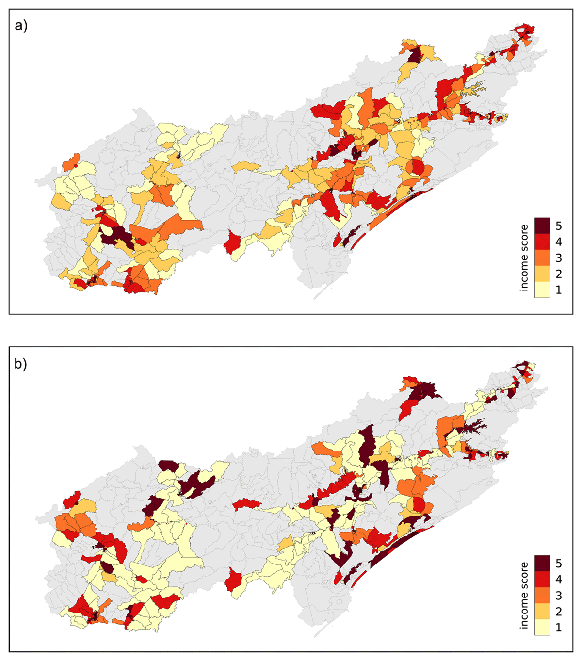
Figure 7
The distribution of income scores for the mode for each census sector is shown for (a) the observed (true) income score, and (b) the predicted income score. The scale ranges from 1 to 5, corresponding to the lowest to highest income score.
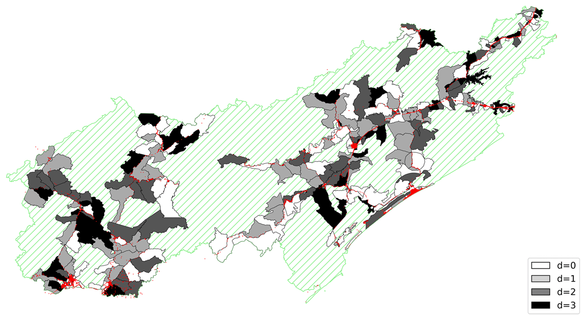
Figure 8
Differences between the real and predicted labels for each census sector of Vale do Ribeira. The grey scale shows the difference between the real and predicted labels (Eq. 3), with d = 3 being a big difference, and d = 0 a perfect match. The red dots represent geolocations for which street images were available. Census sectors for which street imagery was not available are shaded green.
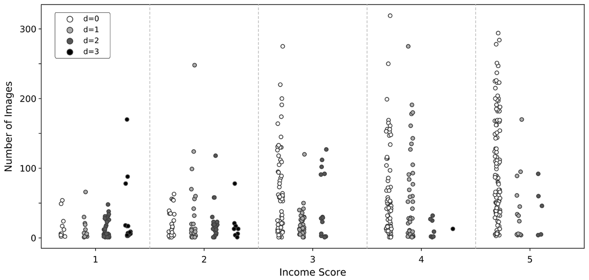
Figure 9
Distribution of predictions by the model indicating the prediction difference of the income score and the number of images per census sector (points). Each income score category includes the 500 census sectors available in Vale do Ribeira. The scale bar shows the difference from 0 (exact match) to 3 (poor match) between the real label and the predicted label (Eq. 3).
Table 3
Prediction results using the test set for each fold. Each column represents a different metric, from left to right the percentage of correctly predicted classes with an error margin of ± 0, ± 1, mean absolute error (MAE), Pearson’s correlation coefficient (r), and Kendall’s Tau rank correlation coefficient (τ).
| ACCURACY ERROR MARGIN (%) | MAE | r | τ | ||
|---|---|---|---|---|---|
| ±0 | ±1 | ||||
| fold 0 | 53 | 78 | 0.21 | 0.74 | 0.30 |
| fold 1 | 55 | 80 | 0.21 | 0.72 | 0.32 |
| fold 2 | 56 | 80 | 0.20 | 0.71 | 0.32 |
| fold 3 | 57 | 81 | 0.23 | 0.67 | 0.34 |
| fold 4 | 56 | 81 | 0.22 | 0.69 | 0.33 |
| Avg fold. | 55 | 80 | 0.21 | 0.71 | 0.32 |
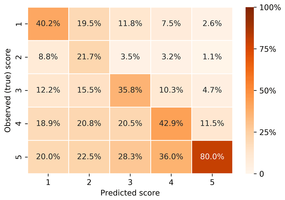
Figure 10
Confusion matrix between observed and predicted income scores. Each cell represents the percentage of the correct predictions. The best case would be a complete diagonal line with perfect accuracy.