
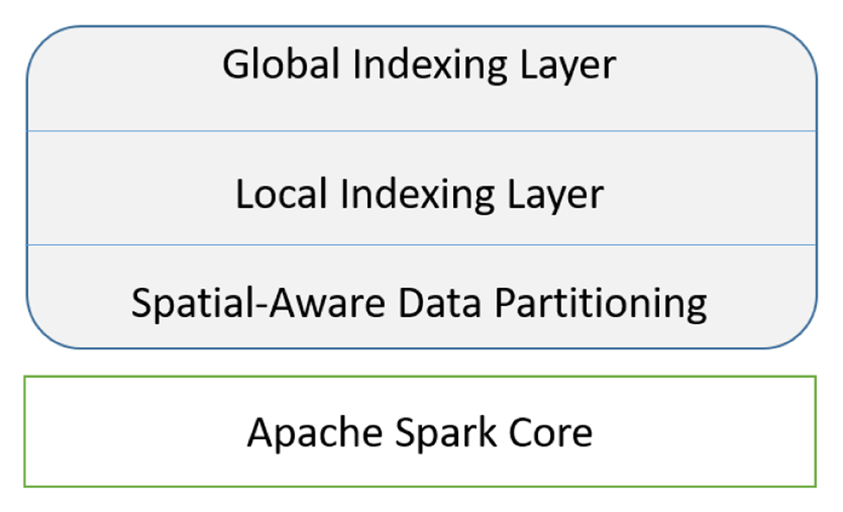
Figure 1
Extension of Spark core to implement SparkNN.
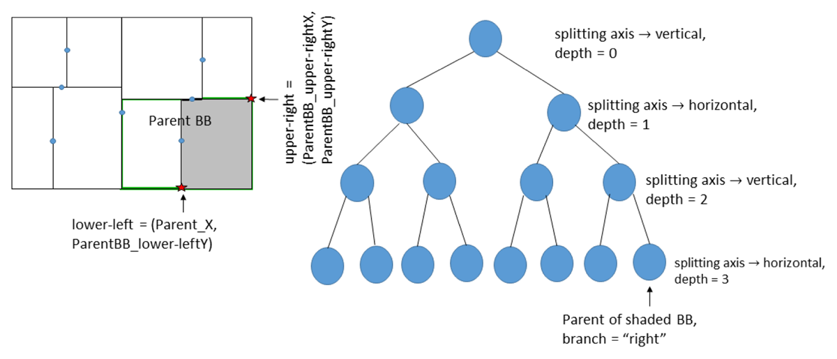
Figure 2
Partitioning the spatial data into BBs.
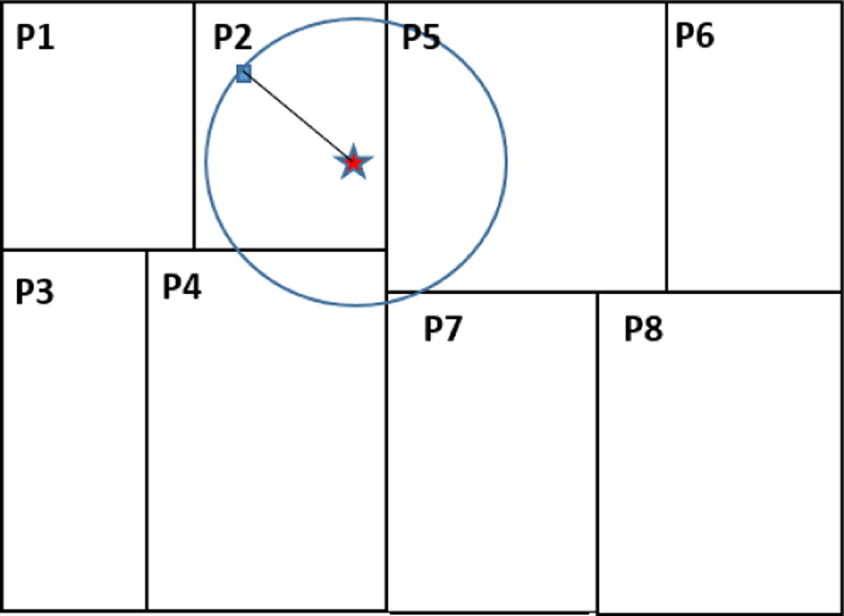
Figure 3
Global indexing of the partitions.
Algorithm 1
kNN from SARDDs.
| Input: node := root of the tree in a RDD partition, needle := {n0, n1, …} the query point, k := an integer value corresponding to the number of nearest neighbors to find |
| Output: bpq := A bounded priority queue containing the k-nearest neighbors |
| Function Knearest (node, needle, k) : |
| Declare bpq as a BoundedPriorityQueue to contain can didate nearest neighbors |
| Set the size of bpq to k |
| Function nearest (node) : |
| default ← node |
| if default == NULL then |
| return NearestPoint |
| else |
| Enqueue default into bpq |
| end |
| if ni ≤ defaulti then |
| NearestPoint ← nearest (left(node)) |
| else |
| NearestPoint ← nearest (right(node)) |
| end |
| if bpq is not full OR |defaulti – ni| < distance(needle, head(bpq)) then |
| if ni ≤ defaulti then |
| NearestPoint ← nearest (right(node)) |
| else |
| NearestPoint ← nearest (left(node)) |
| end |
| return NearestPoint |
| end |
| Knearest (node, needle, k) |
| return bpq |
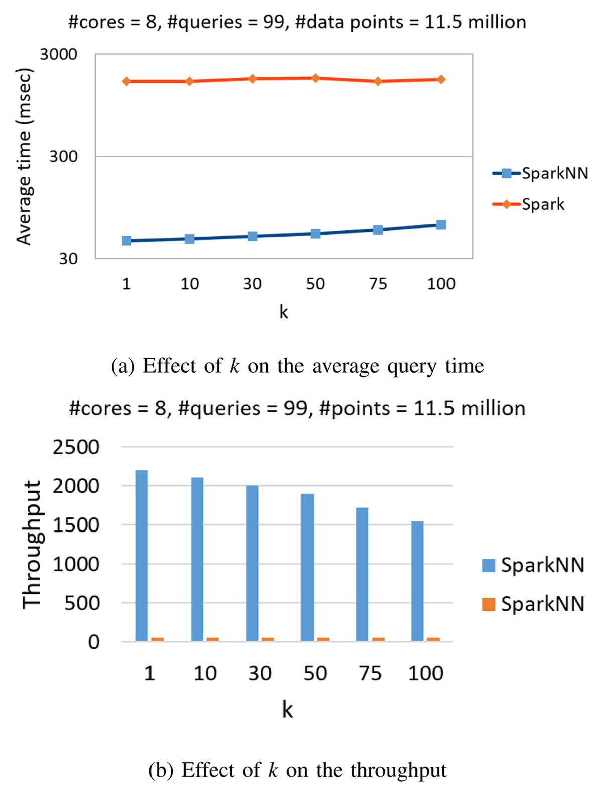
Figure 4
Impact of k.
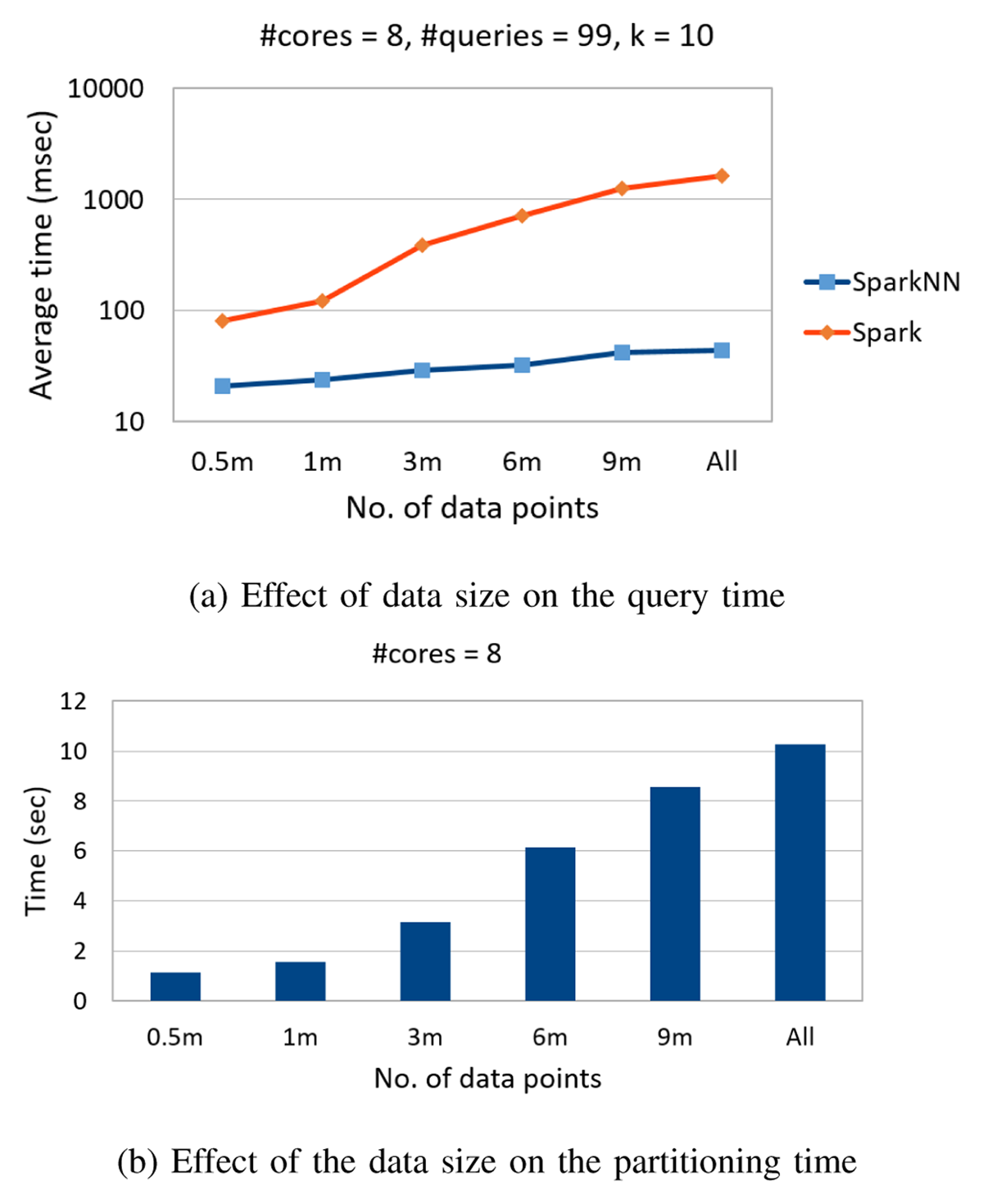
Figure 5
Impact of data size on data load time.
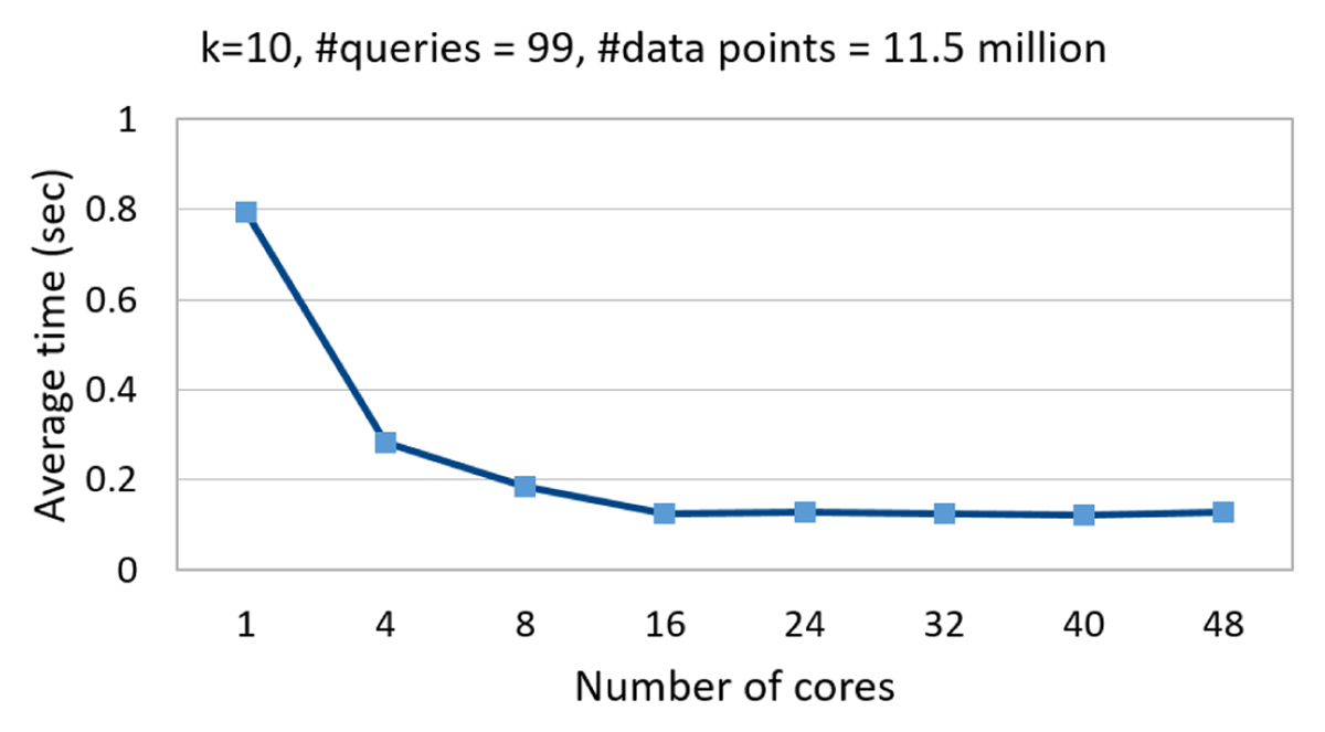
Figure 6
Effect of no. of cores on the scalability of SpakNN.
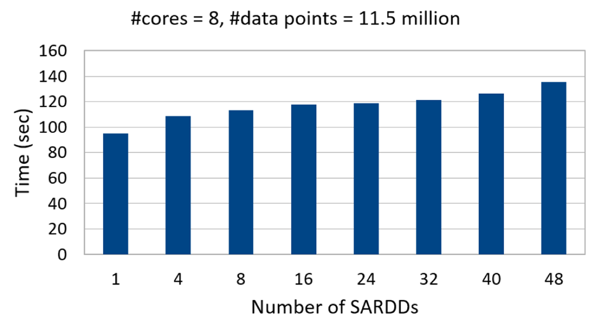
Figure 7
Effect of the number of SARDD on the partitioning time.