
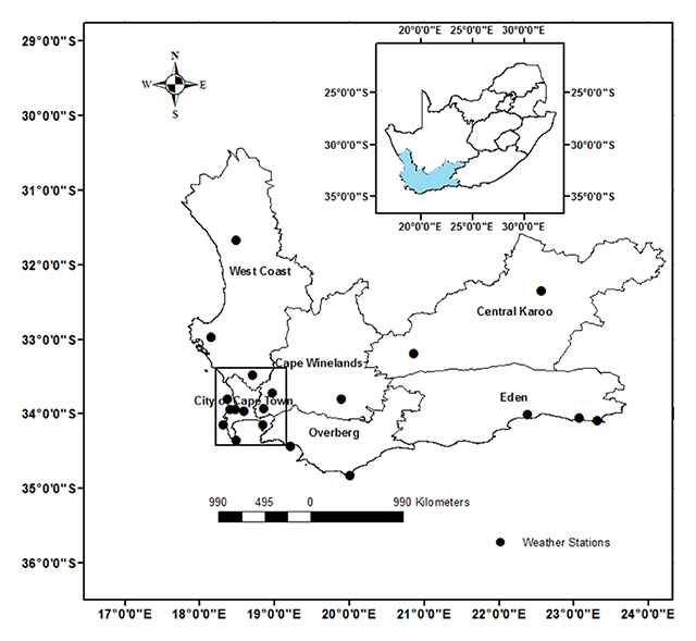
Figure 1
Study Area (square) in Western Cape South Africa with 10 weather stations.
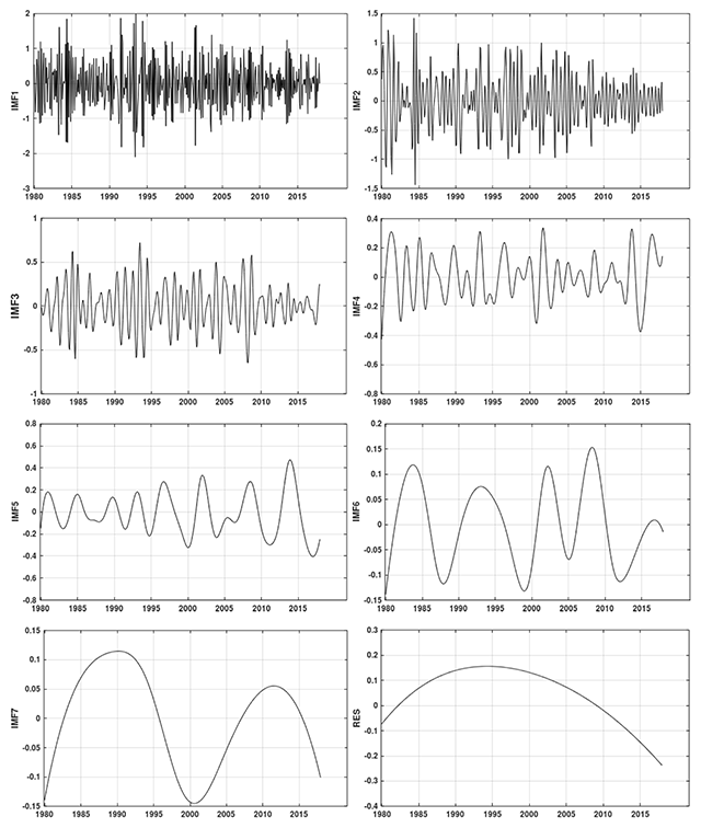
Figure 2
Decomposition of rainfall into IMF1 to 7 and residual using EEMD. The x-axis represents the time in years and y-axis represents the frequency. The graphs are labelled on the y-axis from IMF1 (first graph on the left) to RES (last graph on the bottom right) which is a graph of the residual. IMF1 captures the noise found in the rainfall data, IMF2 inter-annual oscillation, IMF3 annual oscillation, IMF4 2-years oscillation, IMF5 4.5-year oscillation, IMF6 7-year oscillation and IMF7 16.5 year oscillation. The plot of the residual shows the general trend of the rainfall.
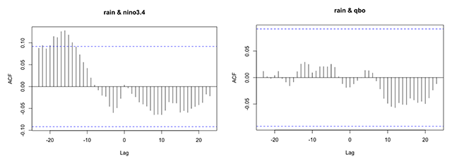
Figure 3
Cross-correlation for rainfall with Niño 3.4 and QBO. The x-axis represents the time gap in months and y-axis represents the correlations. The spikes that are above or below the dotted blue line indicate significant correlation. In the left graph shows that there is correlation of rainfall and Niño 3.4 index at lag –14 to –19. The right graph shows that there is no correlation of rainfall and QBO. The raw data is not showing any association of ENSO and QBO with rainfall data.
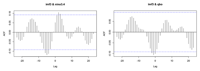
Figure 4
Cross-correlation for IMF3 with Niño 3.4 and QBO. The x-axis represents the time gap in months and y-axis represents the correlations. The spikes that are above or below the blue line indicate significant correlation. In the left graph shows that there is correlation of rainfall’s IMF3 and Niño 3.4 index at lag –4, –5, –6, 2 and 3. The right graph shows that there is correlation of rainfall’s IMF3 and QBO at lag –1 and –2.
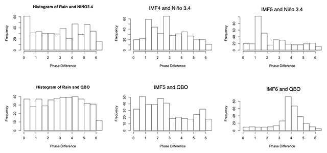
Figure 5
Histogram plot of synchronisation of rainfall, QBO and Niño 3.4 index IMFs. The x-axis represents the phase difference in radians and y-axis represents the frequency. The plots shows a clear peak for rainfall IMF5 with Niño 3.4 IMF5 (top right) which shows that there is phase locking. The last graph on the bottom right is a plot of rainfall’s IMF6 and QBO IMF6 which shows that there is phase locking since there is a clear peak.
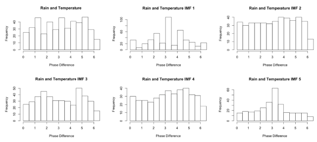
Figure 6
Histogram plot of the synchronisation of rainfall IMFs and temperature IMFs. The x-axis represents the phase difference in radians and y-axis represents the frequency. The plots shows a clear peak for Rainfall and Temperature for IMF1 (second graph on top), and IMF5 (bottom right). This shows that there is phase locking for these IMFs. IMF1 captures the noise in the data and IMF5 captures the 4.5 year-oscillation in the data.