
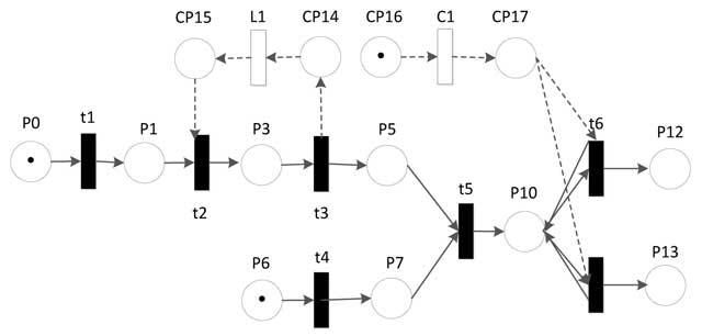
Figure 1
Petri net of a composite web service.
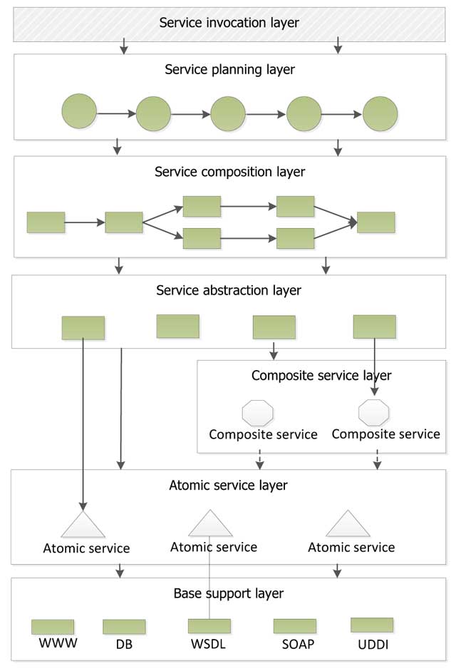
Figure 2
The layered service composition architecture.
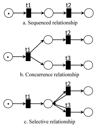
Figure 3
The basic structural relationship among web services.
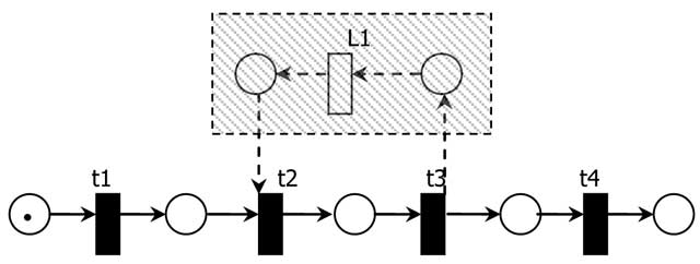
Figure 4
The loop structure.
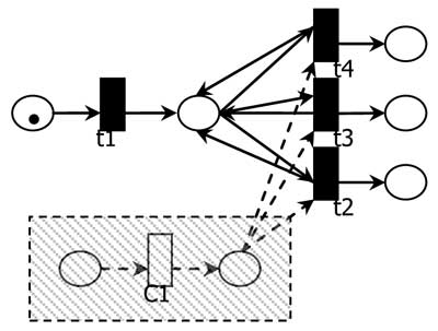
Figure 5
The selective structure with choice conditions.
Table1
The details of computing service.
| ID | web service | Function | Input | Output |
|---|---|---|---|---|
| t1 | AddService | Addition | a;b | e1 |
| t2 | SubstractService | Substraction | c;d | e2 |
| t3 | MultiplicationService | Multiplication | E1;E2 | r |
| t5 | PowerService | Square | r | r1 |
| t6 | AbsService | Absolute value | r | r4 |
| t7 | SinService | Sine | r1 | r2 |
| t8 | CosService | Cosine | R2 | r3 |
| t9 | SqrtService | Square root | r4 | r5 |
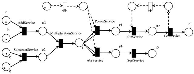
Figure 6
Scientific computing service Petri net.
Table 2
Data association hash table.
| ti:pi | t3:P6 | t3:p7 | t5:P9 | t6: P11 | T7: P13 | t8: P15 | t9: P17 |
| tj:pj | t1:P2 | T2: P5 | t3: P8 | t3:P8 | T5: P10 | t7: P14 | t6: P12 |
Table 3
The mapping table between ID and name.
| ID | P2 | P5 | P6 | p7 | P8 | P9 | P10 | P11 | P12 | P13 | P14 | P15 | P17 |
| name | e1 | e2 | E1 | E2 | r | r | r1 | R | r4 | r1 | r2 | R2 | r4 |
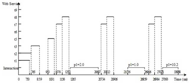
Figure 7
The web services execution time coordinates.
Table 4
The execution result table.
| service ID | Service name | Input name & value | Output name & value |
|---|---|---|---|
| t2 | SubstractService | c(4.0) d(1.0) | e2(3.0) |
| t1 | AddService | a(8.0) b(3.0) | e1(11.0) |
| t3 | MultiplicationService | E1(11.0) E2(3.0) | r(33.0) |
| t5 | PowerService | r(33.0) | r1(1089.0) |
| t7 | SinService | r1(1089.0) | r2(0.9055) |
| t8 | CosService | R2(0.9055) | r3(0.6172) |
| t7 | SinService | r1(1089.0) | r2(0.9055) |
| t8 | CosService | R2(0.9055) | r3(0.6172) |
| t7 | SinService | r1(1089.0) | r2(0.9055) |
| t8 | CosService | R2(0.9055) | r3(0.6172) |