
Table 1
Lesson goals, activity time (tested with up to 25 students) and materials list.
| LESSON GOALS | ACTIVITY TIME | MATERIALS |
|---|---|---|
| Lesson 1 Identify what can be learned from tracking animal movements. Simulate tracking an animal using active and passive acoustic telemetry. | Set up area: 10 min Assign roles: 10 min Brainstorm--Why track animals: 5 min Simulate acoustic telemetry: 20 min | Cardstock to mark activity area Dog tags, lanyards or tape to ID “animals” Optional: Animal face masks (to make the activity festive, we use a Mardi Gras theme). Tables 2 and 3 data sheets, pens, clip boards Assorted games/activities. (We use Perfection, Tic Tac Toe, water bottle flip, money maze puzzles, peg game boards, table top cornhole and 50-piece puzzles). |
| Lesson 2 Recognize the different types of tracking tags available. Determine the appropriate tag to use based on the research question being asked. | Teacher Overview:15 min Activity: 30 min | Pre-activity homework-investigate tag types Information in Figures 3 and 4 Assessment Sheet: Choose the Right Tracking Tool found in online lesson |
| Lesson 3 Gain skills in data analysis by determining the movement ecology of tagged bull sharks. Determine driving factors of observed movement patterns. | Day 1: Teacher Overview: 20 min Students review Range Test results and Elements of Good Data Stewardship: 25 min Day 2: Data Analysis and Reflections 45 min | Pre-activity homework investigating bull shark ecology and the role of phytoplankton in food webs Student access to Figures 5 and 6 Student access to Figures 7, 8, 9 and Table 5 |

Figure 1
Ocean Animals on the Move poster with QR Code linked to three lessons focused on animal telemetry, available at https://gcoos.org/resources/for-educators/.
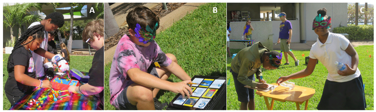
Figure 2
Examples of activities along different paths: a) The game Perfection played with astronaut gloves and a mini grabber tool to simulate a robotic arm; b) Tic-tac-toe board (homemade to contain science information); and c) Bottle flipping challenge.
Table 2
Track Your Classmate Data Sheet: Round 1: Active Acoustics.
| Scientist Identification Number________ Animal Identification Letter________ Start Time ________ End Time________ Location (path selected)________________ | |
| TRANSMITTER TIME INTERVAL | OBSERVATIONS MADE AT EXACT TIME OF “PING” |
| 20 sec | |
| 40 sec | |
| 60 sec | |
| 80 sec | |
| 100 sec | |
| 120 sec | |
| Notable observations made between “pings” | |
Table 3
Track Your Classmate Data Sheet: Round 2: Passive Acoustics.
| “Receiver” Identification Letter______ Start Time________ End Time________ Location (fixed position of receiver)________________ | |
| TRANSMITTER TIME INTERVAL | ANIMAL IDENTIFICATION NUMBERS WITHIN 1 METER OF RECEIVER AT TIME OF “PING” |
| 20 sec | |
| 40 sec | |
| 60 sec | |
| 80 sec | |
| 100 sec | |
| 120 sec | |

Figure 3
Examples of different tag types used in animal movement studies.
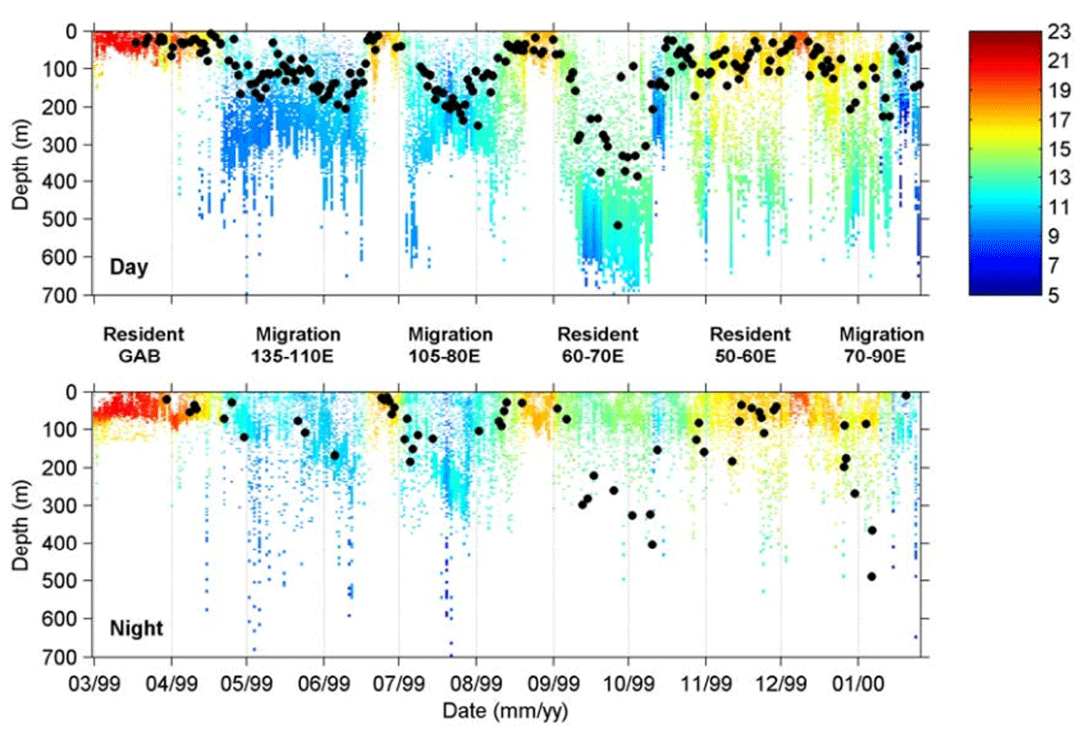
Figure 4
These graphs show the daily daytime (top image) and nighttime (bottom image) patterns of diving and feeding behavior of a southern bluefin tuna during 11 months at sea recorded by an archival tag. The colors indicate water temperature and the black circles indicate a feeding event. Credit: CSIRO Australia.
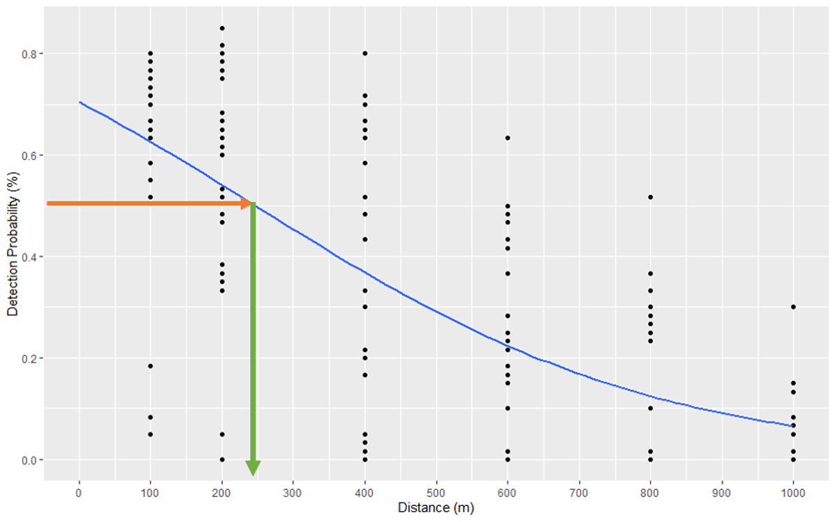
Figure 5
Range test results showing that 50% tag detectability is predicted at a receiver distance of 250 m.
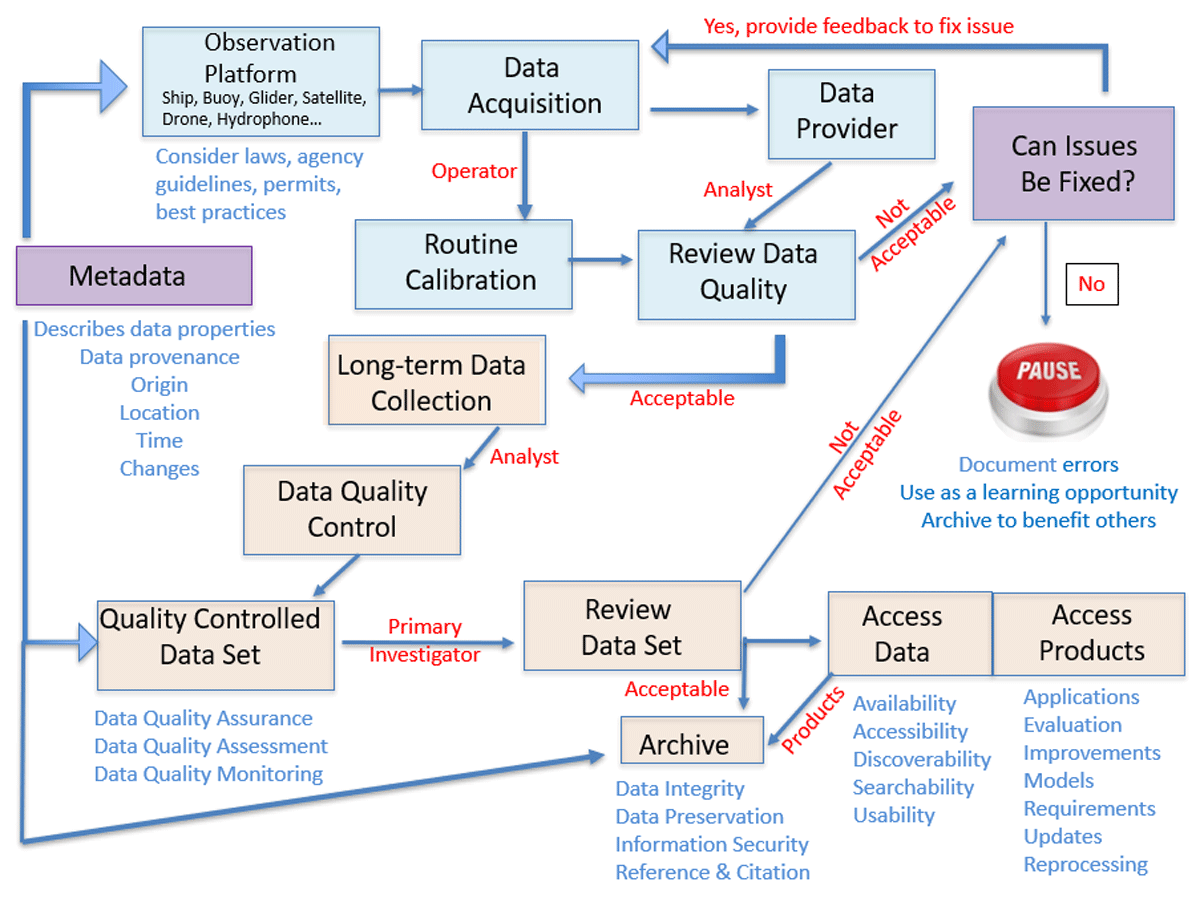
Figure 6
Elements of good data stewardship include metadata and quality control throughout the entire work flow.
Table 4
A typical metadata table used for acoustic tagging projects.
| DATE | TAG ID | TAG TYPE | SPECIES | SEX | LENGTH, CM | LAT/LONG | DEPTH, M | METHOD CAPTURE | NAME |
|---|---|---|---|---|---|---|---|---|---|
| 03112025 | A8–03112025 | Fin | C. leucas | M | 120 | 153.32–27.29 | 15 | Line | M. Rider |
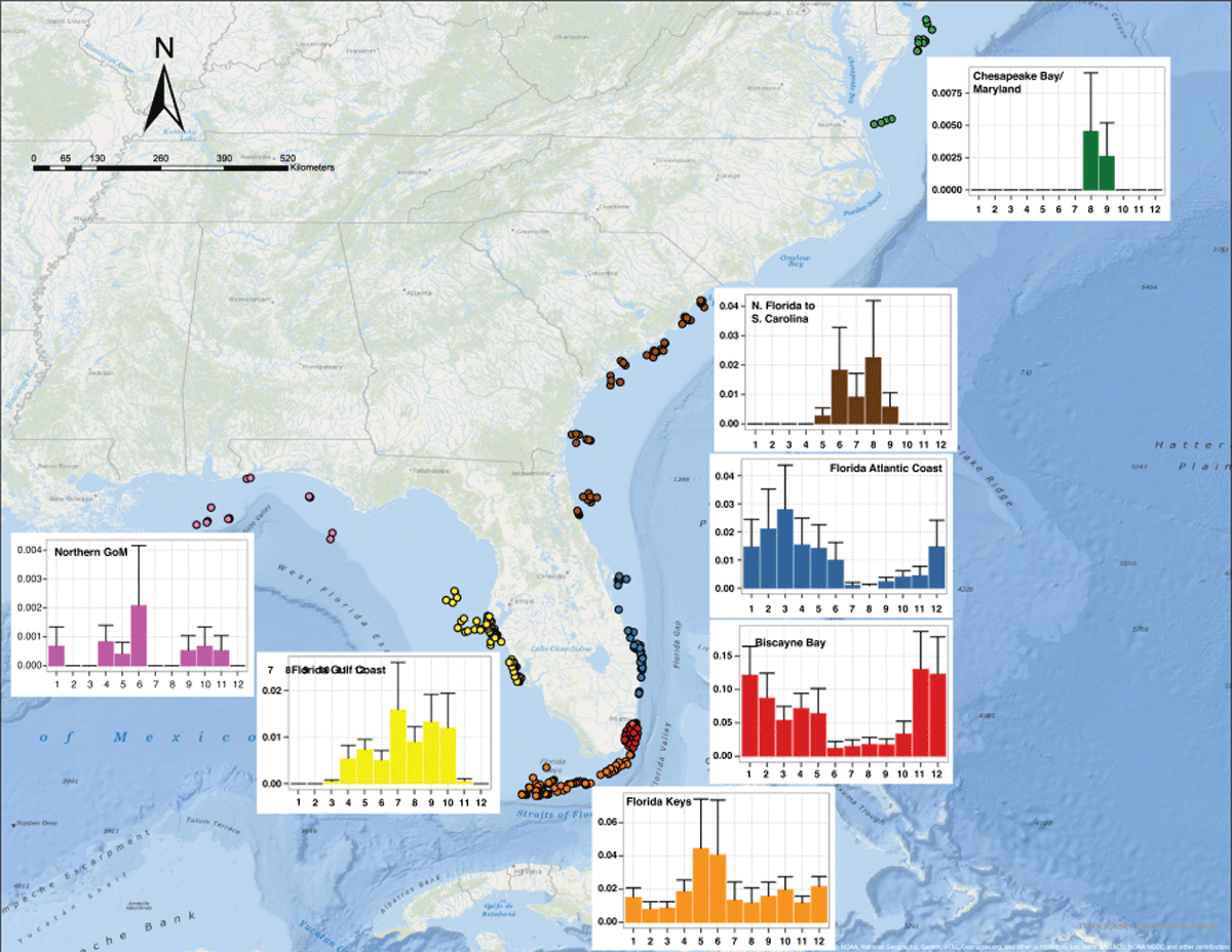
Figure 7
Locations of receivers (color coded by region) with detections of C. leucas originally tagged in Biscayne Bay. Mean residency indices of these sharks (y-axis) are plotted as bars + S.D. over months (x-axis) (January-December, 1–12). Each of the 6 general areas in the study are displayed: Northern Gulf (pink), FL Gulf Coast (yellow), FL Keys (orange), Biscayne Bay (red), FL Atlantic Coast (Blue), Northern FL to SC (brown) and Chesapeake Bay, MD (green).
Table 5
Summary of metadata for acoustically tagged C. leucas individuals detected more than 10 days within the cooperative networks.
| TRANSMITTER ID NUMBER | DATE TAGGED | TAGGING LATITUDE | TAGGING LONGITUDE | SEX | TOTAL LENGTH, CM | LIFE STAGE | DAYS DETECTED | DAYS AT LIBERTY |
|---|---|---|---|---|---|---|---|---|
| 24655 | 02/24/2015 | 25.7480 | –80.1890 | F | 263 | Adult | 161 | 1616 |
| 24660 | 02/27/2015 | 25.7262 | –80.1577 | F | 219 | Subadult | 362 | 1616 |
| 24661 | 02/24/2015 | 25.7262 | –80.1577 | F | 250 | Adult | 88 | 1616 |
| 58396 | 08/11/2015 | 25.7051 | –80.0868 | F | 211 | Subadult | 267 | 1616 |
| 58403 | 01/21/2016 | 25.6220 | –80.1790 | F | 202 | Subadult | 282 | 1588 |
| 13487 | 12/12/2017 | 25.7294 | –80.1581 | F | 196 | Subadult | 233 | 897 |
| 16325 | 03/10/2017 | 25.7289 | –80.2322 | F | 244 | Adult | 240 | 1174 |
| 16324 | 08/13/2017 | 25.6921 | –80.0850 | F | 261 | Adult | 17 | 1018 |
| 16328 | 02/07/2017 | 25.7145 | –80.2082 | M | 196 | Subadult | 21 | 1205 |
| 18401 | 09/11/2016 | 25.6176 | –80.1500 | M | 188 | Juvenile | 15 | 1354 |
| 18413 | 10/17/2016 | 25.6126 | –80.1410 | F | 242 | Adult | 30 | 1318 |
| 18415 | 10/22/2016 | 25.6380 | –80.1968 | F | 191 | Subadult | 268 | 1313 |
| 18419 | 01/20/2017 | 25.6016 | –80.0907 | F | 236 | Adult | 61 | 1223 |
| 18421 | 02/04/2017 | 25.6223 | –80.0980 | F | 242 | Adult | 31 | 1208 |
| 20563 | 12/04/2015 | 25.7002 | –80.9900 | F | 256 | Adult | 90 | 1636 |
| 20773 | 02/16/2016 | 25.7051 | –80.0868 | F | 245 | Adult | 119 | 1562 |
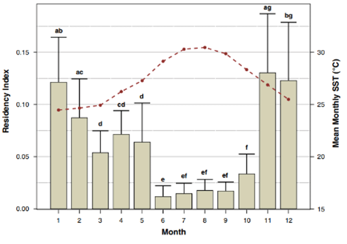
Figure 8
Bars represent mean monthly residencies (+1 standard deviation) of C. leucas within the Biscayne Bay array between June 2015 and June 2020. Bars with the same letter do not significantly differ from one another (P > 0.05). Mean SST (dashed red line) was calculated from average monthly temperatures between 2015 and 2020.
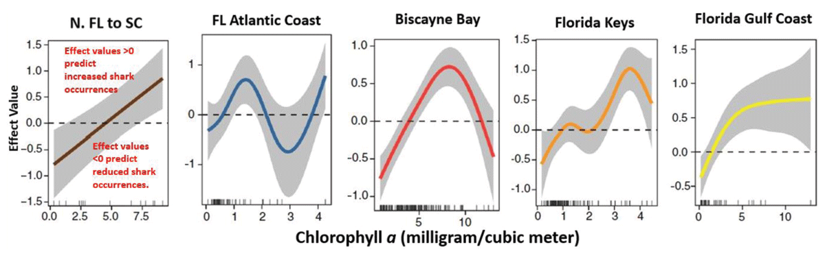
Figure 9
These graphs show the effect of Chlorophyll a on shark detections in each of five study regions. The concentration of Chl a significantly affected the number of days bull sharks were detected at each of the locations.