
Introduction
Biodiversity is critical from the perspective of ecosystem services such as food, oxygen, and socio-economic benefits that support human livelihoods. The 2010 conclusion of the 10-year Census of Marine Life program enhanced our understanding of the diversity, distribution and abundance of life in the ocean (Costello et al. 2010) and made clear the need for a systematic and sustainable approach to monitoring biodiversity across local to global scales to understand how diversity and ecosystems are changing. In response, several federal agencies teamed up with the National Oceanographic Partnership Program (NOPP) to develop an operational US Marine Biodiversity Observation Network (MBON). The plan and recommendations to attain MBON are described in a 2010 workshop report of biodiversity experts (https://cdn.ioos.noaa.gov/media/2017/12/BON_SynthesisReport.pdf). Priorities include: 1) Systematic collection and sharing of marine life information in ways that ensure the information is available for practical application; 2) Integrating historical and current data with new observations to document status and trends in the face of climate- and human-induced change; 3) Using a combination of existing and new tools in the areas of remote sensing, molecular technologies, animal tracking, and environmental research to understand ocean health; and 4) Making information about the relationships between biodiversity, productivity and ecosystem health available for decision making by people and businesses who depend on the ocean.
An overview of three animal telemetry-focused lessons developed using the wealth of publicly available information made available through MBON (https://ioos.noaa.gov/project/mbon/) is the focus of this paper. Authentic data, based on research published by Rider et al. (2021) was used to develop the lessons focused on the method, technology and applications of acoustic telemetry. Movement patterns of bull sharks acoustically tagged in Biscayne Bay, FL, and tracked along the U.S. Southeast Atlantic and Gulf coasts between 2015 and 2020, were the example used to demonstrate how observations of marine life are needed to document status and trends in the face of human- and climate-induced change. The bull shark study is one of few looking at movement patterns over large spatial scales by collaborating across multiple acoustic networks, demonstrating how coordination of acoustic arrays across large spatial scales can enable understanding of movement patterns not previously possible. Over the course of the lessons, students explore how a range test is conducted to determine the placement of receivers at a field site and explore the five “W”s of the study: 1) Who was tagged (22 bull sharks); 2) What was the purpose of tagging (to better understand the movement ecology of bull sharks); 3) Where did they go (from the northern Gulf of Mexico to as far north as Maryland); 4) When did they go (they were tracked year-round, with site-specific patterns emerging); and 5) Why did they go (environmental effects of Sea Surface Temperature (SST) and Chlorophyll a were investigated). The importance of good data stewardship practices and an understanding that the ocean is a vast, interconnected system of species, habitats and ecosystems that rely on one another for balance, resilience and adaptation are important components of the lessons. Table 1 provides a summary of lesson goals, activity times and needed materials.
Table 1
Lesson goals, activity time (tested with up to 25 students) and materials list.
| LESSON GOALS | ACTIVITY TIME | MATERIALS |
|---|---|---|
| Lesson 1 Identify what can be learned from tracking animal movements. Simulate tracking an animal using active and passive acoustic telemetry. | Set up area: 10 min Assign roles: 10 min Brainstorm--Why track animals: 5 min Simulate acoustic telemetry: 20 min | Cardstock to mark activity area Dog tags, lanyards or tape to ID “animals” Optional: Animal face masks (to make the activity festive, we use a Mardi Gras theme). Tables 2 and 3 data sheets, pens, clip boards Assorted games/activities. (We use Perfection, Tic Tac Toe, water bottle flip, money maze puzzles, peg game boards, table top cornhole and 50-piece puzzles). |
| Lesson 2 Recognize the different types of tracking tags available. Determine the appropriate tag to use based on the research question being asked. | Teacher Overview:15 min Activity: 30 min | Pre-activity homework-investigate tag types Information in Figures 3 and 4 Assessment Sheet: Choose the Right Tracking Tool found in online lesson |
| Lesson 3 Gain skills in data analysis by determining the movement ecology of tagged bull sharks. Determine driving factors of observed movement patterns. | Day 1: Teacher Overview: 20 min Students review Range Test results and Elements of Good Data Stewardship: 25 min Day 2: Data Analysis and Reflections 45 min | Pre-activity homework investigating bull shark ecology and the role of phytoplankton in food webs Student access to Figures 5 and 6 Student access to Figures 7, 8, 9 and Table 5 |
About the Ocean Animals on the Move Poster and Lessons: The Ocean Animals on the Move: Using Technology to Track Marine Life poster shown in Figure 1 depicts components of a telemetry system, including different types of tags on a variety of marine animals, fixed (buoy) and mobile (glider) receiver platforms and a satellite with streaming zeros and ones simulating transmission of data. The poster, which contains a QR code linking to the three lessons, is intended to help students visualize elements of an animal tracking system. The digital poster and detailed instructions for each National Education Standards-aligned lesson are available at https://gcoos.org/resources/for-educators/. The overarching goal of the poster and lessons is to educate students about the purpose and process of animal tracking and the data stewardship practices needed to apply the information to real-world challenges. Lessons 1 and 2 introduce students to animal telemetry’s basic concepts and tools. Lesson 3 uses authentic research focused on understanding the movement ecology of bull sharks. Feedback from Grade 5–12 students and educators from ten schools in Pinellas County, Florida, is incorporated into the lessons. Lessons 1 and 2 proved most suitable for Grade 8–12 students while Lesson 3, because of the complex nature of primary production, ecosystem interactions and environmental factors, was found to be most appropriate for upper level high school students.
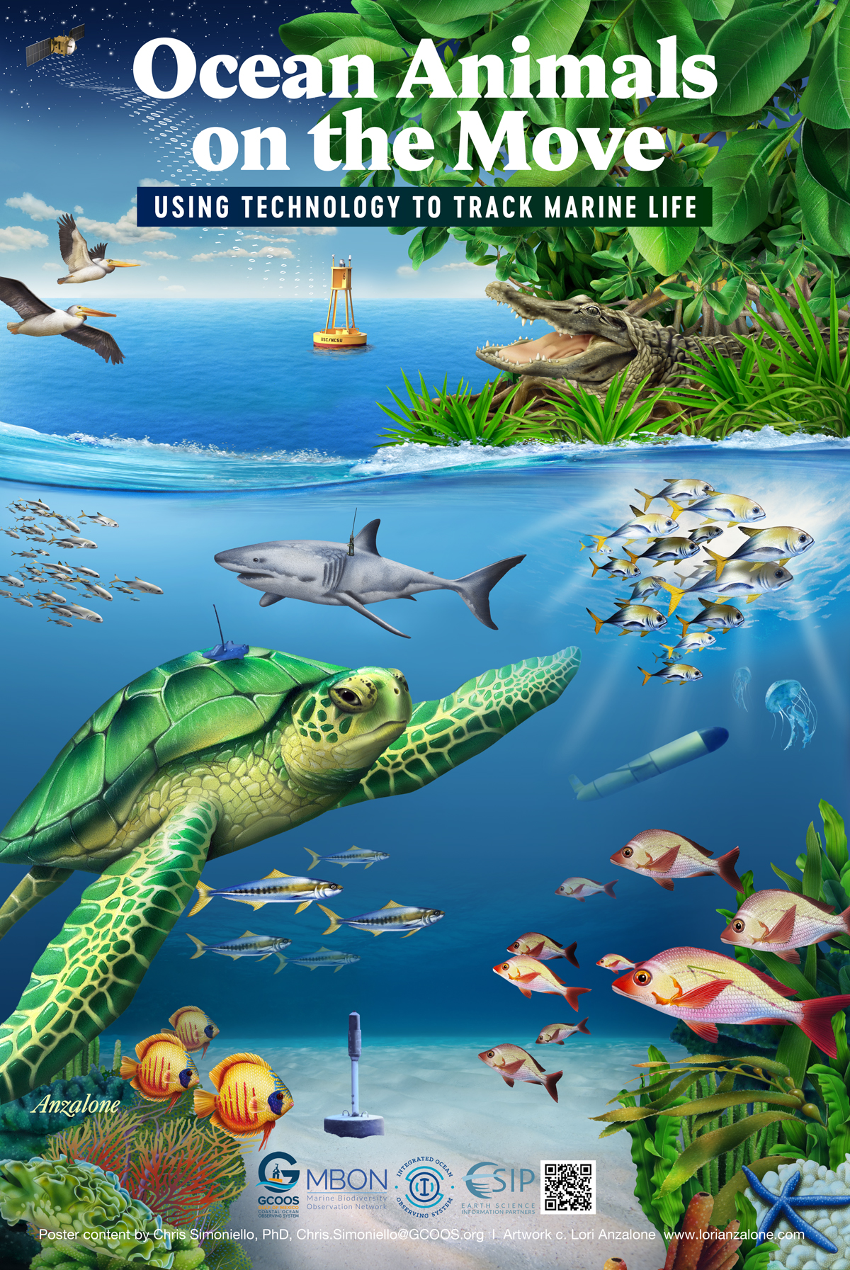
Figure 1
Ocean Animals on the Move poster with QR Code linked to three lessons focused on animal telemetry, available at https://gcoos.org/resources/for-educators/.
About the U.S. Animal Telemetry Network (ATN): An integral tool in understanding the distributions of marine species over space and time is animal telemetry—the science of gathering information on the movement and behavior of marine organisms using animal-borne sensors (i.e., tags). Over time, a combination of animal movement and oceanographic data like ocean temperature, chlorophyll distribution (an indicator of primary production), and currents can bring to light the forces driving the observed movements. For example, they can shed light on an animal’s range, use of different habitats, foraging behavior and migration corridors (Allen & Singh 2016; Costa et al. 2010; Aarts et al. 2008). As tags have decreased in size, researchers have been able to study animals ranging from six-gram salmon smolts to 150-ton whales and everything in between. In addition, the capabilities of telemetry tag sensors have grown so that we are able to capture not only data about their movements but also information about the animal (e.g., body temperature, heart rate), its behavior (e.g., vocalizations, breathing), and data on their environment such as water temperature and salinity (Sandrelli et al. 2025; Jónsdóttir et al. 2024; Korus et al. 2024; Goldbogen et al. 2019). Animal telemetry data and associated oceanographic data sets from a wide variety of species and platforms are openly available at https://ioos.noaa.gov/project/atn/.
Overview of Ocean Animals on the Move Lessons
Lesson 1 Overview: Introduction to Animal Tracking: Track Your Classmate
The goals of Lesson 1 are to: 1) Have students identify what can be learned from tracking animal movements in the ocean; and 2) Simulate field work that requires tracking an animal using active and passive acoustic telemetry technologies.
Data acquisition from both active and passive acoustics is investigated in Lesson 1 to learn about the types of information that animal tracking from mobile (i.e., ships, autonomous underwater vehicles) and fixed platforms can and cannot provide. Prior to students arriving for the activity, a space with multiple path options is created. The activity was tested in outdoor, cafeteria and traditional classroom settings, with outdoor spaces being preferred by both students and teachers. Each path is designated with a unique name and offers a variety of fun activities (Figure 2) along the way to encourage students to spread out as they select and move along the different paths. If discussions about the concept of “hotspots” or places where animals tend to aggregate in the ocean are desired, the setup should include an especially desirable incentive along one of the paths (e.g., candy, homework pass). Students are paired such that one is the scientist and the other is the animal being tracked. Scientists are assigned a unique number designation and each animal a unique letter designation. If there is an uneven number of students, there should be more animals than scientists.

Figure 2
Examples of activities along different paths: a) The game Perfection played with astronaut gloves and a mini grabber tool to simulate a robotic arm; b) Tic-tac-toe board (homemade to contain science information); and c) Bottle flipping challenge.
Active Acoustic Tracking
Students are gathered in an area away from the activity space and three basic rules of engagement provided: 1) For practical reasons, once an animal starts down a path, they must complete that path before starting down another; 2) There is no talking between scientist/animal partners; and 3) It is ok for scientists to talk with each other and for the animals to interact amongst themselves. Capturing a variety of interactions is ideal. The teacher then explains that a designated time keeper will signal the group (i.e., transmitter pings) at 20 second intervals over the course of two minutes. The scientists will enter on their data sheets (Table 2) the behaviors they observe exactly at the time they hear the signal. At the start of the activity, scientists fill in their identification number, partner animal’s identification letter and start time. Then start the round by signaling the animals to select a path and for the scientists to follow their designated partner(s). Scientists also record the path selected on their data sheets and note the time the last observation is recorded. There is a place on the bottom of the data sheet to record noteworthy observations that take place between the 20 sec intervals. This will demonstrate behaviors not captured by acoustic receivers when tagged animals are out of range or between pings.
Table 2
Track Your Classmate Data Sheet: Round 1: Active Acoustics.
| Scientist Identification Number________ Animal Identification Letter________ Start Time ________ End Time________ Location (path selected)________________ | |
| TRANSMITTER TIME INTERVAL | OBSERVATIONS MADE AT EXACT TIME OF “PING” |
| 20 sec | |
| 40 sec | |
| 60 sec | |
| 80 sec | |
| 100 sec | |
| 120 sec | |
| Notable observations made between “pings” | |
Passive Acoustic Tracking
Scientists and animals now reverse roles. Instead of actively following animals, the scientists will disperse over the activity area and remain in fixed positions (i.e., they become stationary acoustic receivers) for the two-minute duration of the activity. The designated time keeper will once again indicate “start” and signal the group every 20 seconds for two minutes. Animals will move through the activity. At the 20 second intervals, the scientists (i.e., receivers) record on their data sheet (Table 3) the individual numbers of the animals that are within 1 meter of them at the exact moment they hear the “ping”. They will not record any information about behavior and should enter a “0” if no animals are present at the time of the ping. This will allow later discussions about the concept of a “zero value” meaning “no animal present” vs “no data” meaning an animal is possibly present but not detected due to a problem with a tag or receiver.
Table 3
Track Your Classmate Data Sheet: Round 2: Passive Acoustics.
| “Receiver” Identification Letter______ Start Time________ End Time________ Location (fixed position of receiver)________________ | |
| TRANSMITTER TIME INTERVAL | ANIMAL IDENTIFICATION NUMBERS WITHIN 1 METER OF RECEIVER AT TIME OF “PING” |
| 20 sec | |
| 40 sec | |
| 60 sec | |
| 80 sec | |
| 100 sec | |
| 120 sec | |
Track Your Classmate Activity Key Discussion Points
There are benefits and challenges of actively tracking tagged animals from mobile platforms vs. using receivers in a fixed location. Topics for discussion include the cost of each method, the scale of coverage over space and time, and choosing between high resolution information for one animal vs. less detailed information about many. What did the students note in their data sheets? Were there especially desirable locations where students gathered during the activity? If so, what are possible explanations? In nature, hotspots are places where many animals tend to aggregate because of preferred conditions such as food, shelter, favorable currents or water temperature. Scientists use movement data to understand where the animals go, how much time they spend in an area, how they use the habitat (e.g., for feeding, breeding, resting, migrating) and who/what they interact with. The information informs management and sheds light on if/how changing environmental conditions are impacting different species and ecosystems.
Many types of interactions take place during the activity—some can be detected using acoustic telemetry and others cannot. What did students observe between animals, between animals and scientists and between animals and the habitat? Were there noteworthy observations that took place between the 20-second “transmitter ping” intervals? For a scientist trying to understand animal movement ecology, a lot happens between tag detections. Depending on the movement and behavioral information needed to address the research question, acoustic telemetry might not be the best option. Other tracking options are discussed in Lesson 2.
Understanding the relevance of animal tracking is a key point of Lesson 1. Different organizations must make decisions about how to use and protect natural resources in responsible and sustainable ways. Laws guide these decisions. Understanding how different species interact with each other, the environment and other species is critical to their protection. A few examples of stakeholders and how they might apply animal tracking data include: 1) NOAA scientists need to know where and when Highly Migratory Species like Atlantic bluefin tuna spawn so they can regulate fishing at those times and locations; 2) Port managers need to know if sediment kicked up during dredging operations is making the habitat dangerous for threatened or endangered plants and animals; 3) Industries scoping locations for things like offshore aquaculture and offshore wind farms require environmental impact assessments to understand what’s there, how species use the environment, and how proposed activities might impact them; and 4) The military needs to know how ocean noise pollution generated from activities such as seismic surveys, demolition, explosives and sonar might impact protected species before operations can take place. To assess understanding, students are asked to identify a real-world issue that would benefit from using animal tracking technology. Who needs the information and what decision would be made based on the data? Ideas to explore include setting fisheries catch limits and seasons; establishment of marine protected areas; port expansion projects; coastal development; coastal restoration; establishment of commercial navigation routes; scoping offshore energy sites or aquaculture facilities; siting for artificial reef construction; site determination for an eco-tourism business; and understanding climate change impacts to marine life. Students should demonstrate understanding about the animals that need to be tracked, expectations about what could be learned from the data and be aware of supporting information such as environmental and/or socioeconomic data that might be needed.
Lesson 2 Overview: Animal Tracking Tools and Technology
The goals of Lesson 2 are to: 1) Recognize the different types of tags available; and 2) Determine the appropriate tag to use based on the research question being asked.
Introduction to Tracking Techniques: Tagging animals requires a skilled team that can work cooperatively and efficiently to keep people and animals safe; animal ethics training to participate in field and lab work; and permits to conduct field work. There are different types of tracking techniques (Figure 3), each with different benefits, challenges and costs. Finding the right tool for the job is important.
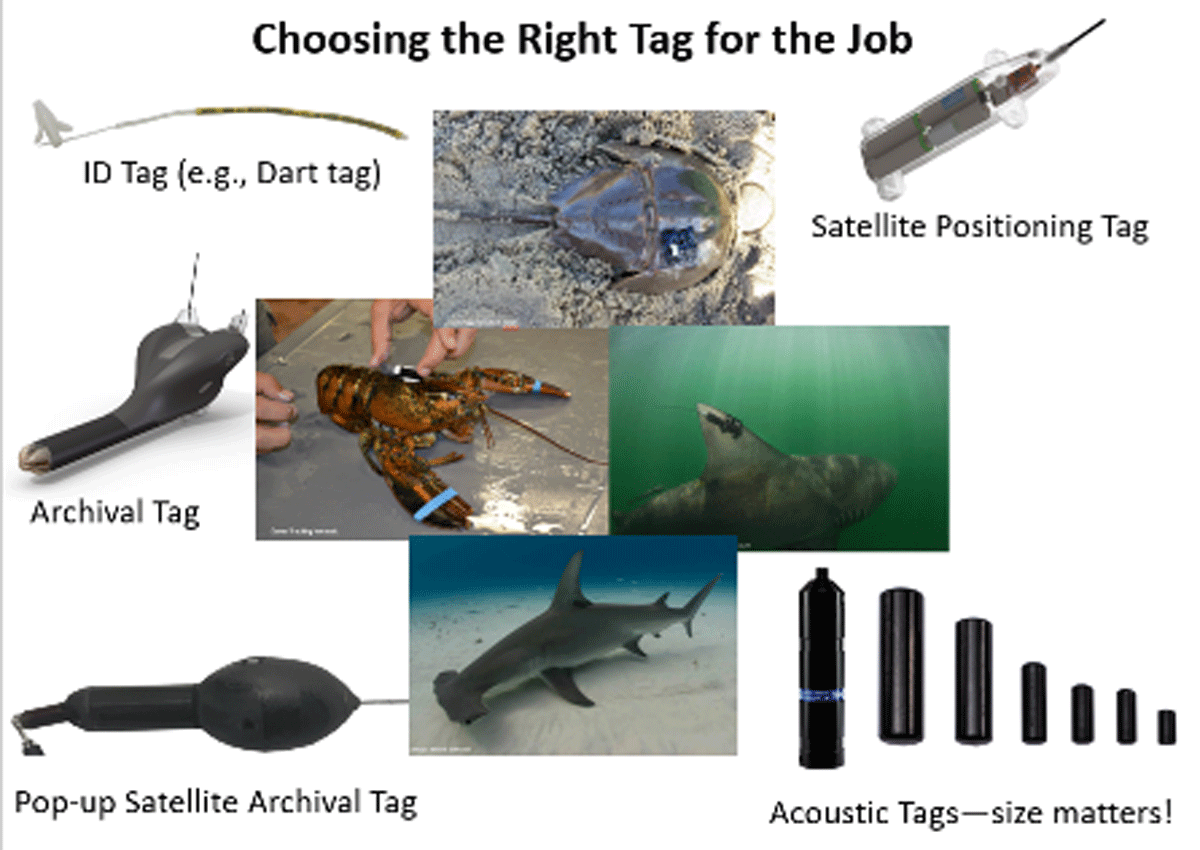
Figure 3
Examples of different tag types used in animal movement studies.
Activity and Assessment: Choose the Right Tracking Tool: In Lesson 2, students are asked to consider multiple factors to select the most appropriate tracking method based on scenarios provided or ones they create. If not familiar with the animals provided, do some fact-finding first. Topics to consider include balancing matters of cost—for tags themselves and operational costs, life style of species, the resolution of information needed, and the frequency and duration of data needed. Examples of scenarios include: 1) The Marine Mammal Commission needs to determine the seasonal migratory routes of gray whales to establish shipping routes that will avoid collisions; 2) Before a coral reef restoration project can proceed, scientists need to know the percent of time that nurse sharks, a near-bottom species, spend in a particular area of the reef; 3) A fish hatchery wants to distinguish between wild and hatchery-released sea trout that are caught by commercial fishermen; and 4) NOAA Fisheries is trying to determine how much time leatherback sea turtles spend at different depths in a foraging area off Nantucket so they can determine possible interactions with lobster pots.
Mark and Recapture: Mark and recapture requires capturing a number of animals, marking them, releasing them back into the population, and then determining the ratio (proportion of marked to unmarked animals) of the population when marked and unmarked animals are captured at a later date. Originally developed to determine growth rate and estimate population size, mark and recapture is also used for the estimation of birth, mortality and emigration rates within populations. Identification tags like the Dart Tag shown in Figure 3 are one of the most basic tools used to mark animals. Each dart has a unique number so that an individual animal with a tag can be identified. If/when a tagged animal is recaptured, we can see where it moved and measure how much it has grown since it was first caught and tagged.
Archival Tags: Archival tags are small data loggers that record dates, times, swim depths, water temperatures, body temperatures and light levels. They can record data every few seconds for up to 10 years, depending on the tags’ sampling frequency and battery life. Archival tags can be attached to the animal externally or internally and must be retrieved for their data to be downloaded. They are used most commonly on species that have a high likelihood of recapture – either through fishing, or upon return visits to breeding and feeding grounds – such as fish, seabirds, sea turtles and marine mammals. An example of the type of information gleaned from an archival tag on a southern bluefin tuna is shown in Figure 4.
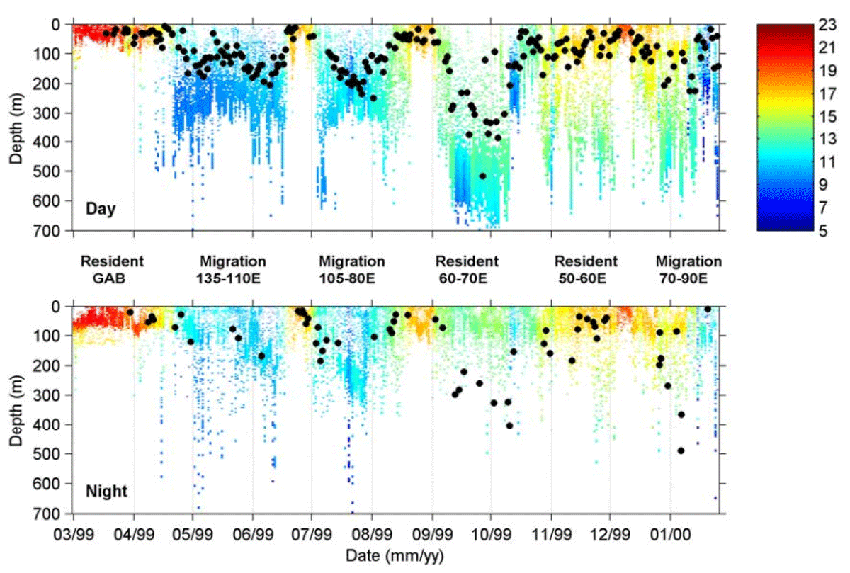
Figure 4
These graphs show the daily daytime (top image) and nighttime (bottom image) patterns of diving and feeding behavior of a southern bluefin tuna during 11 months at sea recorded by an archival tag. The colors indicate water temperature and the black circles indicate a feeding event. Credit: CSIRO Australia.
Pop-up satellite archival tags: Pop-up archival transmitting (PAT) tags are externally placed tags that are pre-set to detach from the animal, rise to the surface and transmit data by radio to the Argos satellite network. This network collects, processes and disseminates environmental data, and has a special channel dedicated to wildlife telemetry. PAT tags provide a means of collecting fishery-independent data (i.e., data collected separately from commercial fishing activities to provide a less biased view of fish populations), and have been deployed on animals such as tuna, marlin, sharks and sea turtles. An example of their use is a study by Jorgensen et al. (2010) that elucidated migration corridors of white sharks (Carcharodon carcharias). Those tagged in South Africa were shown to exhibit return breeding migrations to Australia and individuals tagged off California migrated as far as the Hawaiian Islands. Building a picture of regularly used white shark migration routes can help to reduce the incidental capture of this threatened species by commercial fisheries and minimize undesirable interactions with humans.
Acoustic Tags: Acoustic tags can be attached to an animal externally or internally. They transmit a unique sound signal that identifies the tagged individual when it is within range of a fixed receiving instrument (passive acoustics), usually on the seabed, or a hydrophone operated from a mobile platform (active acoustics) like a vessel or autonomous underwater vehicle. They also can transmit data on swim speed (with an accelerometer) and environmental characteristics such as water temperature and depth. Acoustic tags commonly are used to record the extent to which an animal uses a particular area and to determine how this behavior may change over time. They are suited to research on any species to which a transmitter can be attached or implanted without modifying its behavior such as fish, sharks, crustaceans and squid. Acoustic receivers, or ‘listening stations’, can record the presence of hundreds of animals tagged with acoustic transmitters with a location accuracy of about one meter. Detection ranges can be extended to hundreds of kilometers by placing multiple receivers in grids or lines called arrays. In general, the tag selected should weigh no more than 2.5% of an animal’s body mass. For example, for a 4.5 kg (10 lb) grouper, the heaviest tag you should use is 113 grams (0.25 lb). Smaller tags generally cost less but larger tags produce a stronger signal making detection more likely and typically have batteries with a longer lifespan. Tag technology is advancing all the time. A Predation Detection Acoustic Tag has a unique digestible fuse. Stomach enzymes in the predatory fish break down the fuse. This alters the tag’s signal so that researchers know the transmission signal is now from the predator, not the original animal tagged (Shorgan et al. 2024)!
Lesson 3 Overview: Using Passive Acoustic Telemetry to Study the Movement Ecology of Bull Sharks
The goals of Lesson 3 are to: 1) Gain skills in data analysis by determining the movement ecology of tagged bull sharks throughout the study region; and 2) Determine potential driving factors to explain the movement patterns observed.
Lesson 3 is based on research that used passive acoustic telemetry to study bull shark (Carcharhius leucas) movement along the US Southeast Atlantic and Gulf coasts over space and time (Rider et al. 2021). The processes of field observations, data collection, data curation and stewardship, and analysis that requires critical thinking skills are explored. Content here requires an understanding of food webs, primary production and the role of chlorophyll in marine ecosystems. Beta testing of this lesson led to the conclusion that it is best suited to older students in Grades 10–12.
Introduction to the Research: Sharks tagged in Biscayne Bay, FL, were tracked using an array of receivers (n = 504 individual receivers) operated by multiple researchers as part of a cooperative acoustic tracking network, specifically, the Ocean Tracking Network (Iverson et al. 2019), the Integrated Tracking of Aquatic Animals in the Gulf of Mexico (iTAG, Currier et al. 2015), and the Florida Atlantic Coast Telemetry (FACT, Young et al. 2020) network. Overall, 22 bull sharks were tagged and tracked between March 2015 and June 2020. Before tagging animals, the team determined how and where to set up the receiver stations. Several questions had to be addressed. These included: 1) What is the water depth at the location of interest; 2) What method of receiver deployment is needed; 3) Do local conditions like strong waves and currents require a structure to be built to anchor the receiver; and 4) How will local conditions affect signal detection? To address the latter, a range test of the tracking equipment was required.
Range Testing: Range testing is done on a subset of receivers to determine the distance that transmitted signals (“pings”) from a tag will be picked up by a receiver under local conditions. This is important because parameters like current speed, tidal range, anthropogenic noises and other oceanographic conditions affect sound detection (O’Brien & Secor 2021). In the example here, researchers used sentinel range testing tags with a transmitter rate of one ping per minute, deployed at six distances from the receiver: 100, 200, 400, 600, 800 and 1000 meters. Testing was done for a total of 24 hours after which detection data were downloaded from the receiver and the rate of detections calculated for each distance using the equation
Because the testing tags were set to a rate of one ping per minute, a receiver could have theoretically received a maximum of N = 60 signals in an hour. These proportions were then plotted against their associated distance and a logistic regression curve was fitted to the data points. As part of Lesson 3 activities, students are asked information about the curve, including determining the distance at which 50% of detections are predicted to be received (Figure 5).
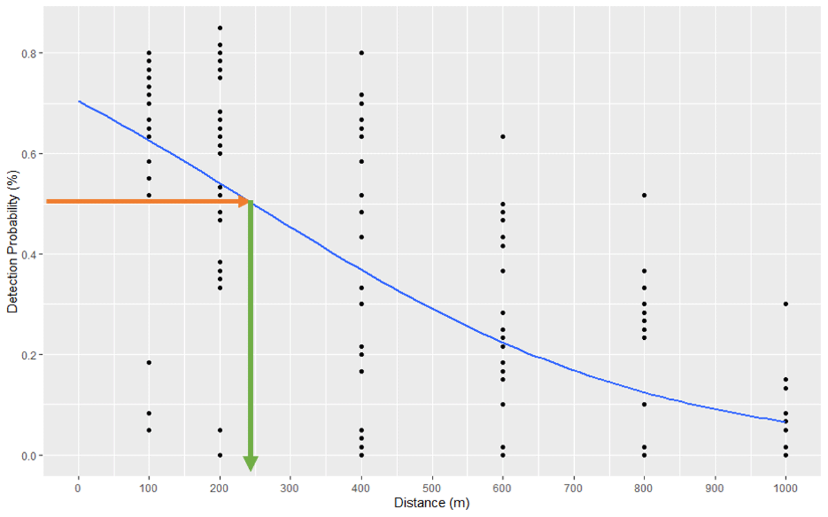
Figure 5
Range test results showing that 50% tag detectability is predicted at a receiver distance of 250 m.
Data Stewardship: Good data stewardship essential for animal tracking studies includes elements shown in Figure 6. Metadata, information about a data set that answers the “who, what, when, where, why and how” of the information provided, is an essential component of the data flow because it provides the context in which information can be used. For example, without a location or time stamp for a receiver, the transmission detections would be meaningless. The words selected to describe a project’s metadata are also important because they become the terms used when people search for information.
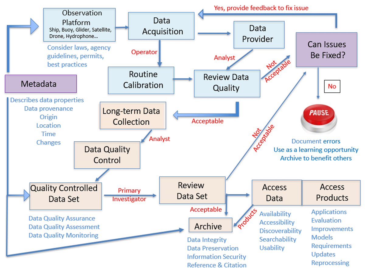
Figure 6
Elements of good data stewardship include metadata and quality control throughout the entire work flow.
Table 4 shows typical metadata used for acoustic tagging projects. Unique tag number(s), type of tag(s), species, sex, length, date of tagging, location, depth and method of capture, and contact details for the person tagging the animal(s) are essential for all tagged animals. In this lesson, students must refer to project metadata to formulate explanations about observed shark movements. Additionally, information about equipment malfunctions must be noted. Without this quality check, it would be impossible to know if a gap in signal detection really means the absence of a tagged animal or is the result of a detection problem, in which case, the residence times of sharks could not be accurately compared between sites.
Table 4
A typical metadata table used for acoustic tagging projects.
| DATE | TAG ID | TAG TYPE | SPECIES | SEX | LENGTH, CM | LAT/LONG | DEPTH, M | METHOD CAPTURE | NAME |
|---|---|---|---|---|---|---|---|---|---|
| 03112025 | A8–03112025 | Fin | C. leucas | M | 120 | 153.32–27.29 | 15 | Line | M. Rider |
Student Analysis of Project Data: Students analyze graphic depictions of movement data to discover that residence indices were lowest in the Biscayne Bay array location during spring and summer months. At this time, other areas, including the Florida Keys, Florida Gulf Coast, and North Florida to South Carolina array locations reached their peak values. However, the lowest residency indices in Biscayne Bay were still higher than the highest values of the other locations (Figure 7).

Figure 7
Locations of receivers (color coded by region) with detections of C. leucas originally tagged in Biscayne Bay. Mean residency indices of these sharks (y-axis) are plotted as bars + S.D. over months (x-axis) (January-December, 1–12). Each of the 6 general areas in the study are displayed: Northern Gulf (pink), FL Gulf Coast (yellow), FL Keys (orange), Biscayne Bay (red), FL Atlantic Coast (Blue), Northern FL to SC (brown) and Chesapeake Bay, MD (green).
Data tables and graphs from the study are also used by students to answer specific questions such as determining the average number of days female sharks were detected over the course of the study compared to male sharks; percent of bull sharks that undertook round trips to various locations and for various durations; identifying the tagged sharks that were detected in the most regions; and figuring out the longitudinal and latitudinal extremes the sharks traveled. Metadata shown in Table 5 is used by the students to formulate ideas about how sample size, life stages and other variables might explain the movement observations.
Table 5
Summary of metadata for acoustically tagged C. leucas individuals detected more than 10 days within the cooperative networks.
| TRANSMITTER ID NUMBER | DATE TAGGED | TAGGING LATITUDE | TAGGING LONGITUDE | SEX | TOTAL LENGTH, CM | LIFE STAGE | DAYS DETECTED | DAYS AT LIBERTY |
|---|---|---|---|---|---|---|---|---|
| 24655 | 02/24/2015 | 25.7480 | –80.1890 | F | 263 | Adult | 161 | 1616 |
| 24660 | 02/27/2015 | 25.7262 | –80.1577 | F | 219 | Subadult | 362 | 1616 |
| 24661 | 02/24/2015 | 25.7262 | –80.1577 | F | 250 | Adult | 88 | 1616 |
| 58396 | 08/11/2015 | 25.7051 | –80.0868 | F | 211 | Subadult | 267 | 1616 |
| 58403 | 01/21/2016 | 25.6220 | –80.1790 | F | 202 | Subadult | 282 | 1588 |
| 13487 | 12/12/2017 | 25.7294 | –80.1581 | F | 196 | Subadult | 233 | 897 |
| 16325 | 03/10/2017 | 25.7289 | –80.2322 | F | 244 | Adult | 240 | 1174 |
| 16324 | 08/13/2017 | 25.6921 | –80.0850 | F | 261 | Adult | 17 | 1018 |
| 16328 | 02/07/2017 | 25.7145 | –80.2082 | M | 196 | Subadult | 21 | 1205 |
| 18401 | 09/11/2016 | 25.6176 | –80.1500 | M | 188 | Juvenile | 15 | 1354 |
| 18413 | 10/17/2016 | 25.6126 | –80.1410 | F | 242 | Adult | 30 | 1318 |
| 18415 | 10/22/2016 | 25.6380 | –80.1968 | F | 191 | Subadult | 268 | 1313 |
| 18419 | 01/20/2017 | 25.6016 | –80.0907 | F | 236 | Adult | 61 | 1223 |
| 18421 | 02/04/2017 | 25.6223 | –80.0980 | F | 242 | Adult | 31 | 1208 |
| 20563 | 12/04/2015 | 25.7002 | –80.9900 | F | 256 | Adult | 90 | 1636 |
| 20773 | 02/16/2016 | 25.7051 | –80.0868 | F | 245 | Adult | 119 | 1562 |
Data Tools of the Research Analysis: Once the research team determined “when and where” the tagged bull sharks were moving, the next question was “why”. Data science tools were used to analyze a variety of environmental variables. One such tool is R, an advanced language that performs complex statistical computations and can interpret data in a graphical form. Here, an R package was used to extract from a variety of websites sea surface temperature (SST) and Chlorophyll a (Chl a) data corresponding to the times and locations of the tagged sharks.
Environmental Factors: The relationship between bull shark residence times in Biscayne Bay and temperature depicted in Figure 8 shows that the highest mean residencies occurred between November and February when mean monthly SST was lower (24.5–26.8C). SST >27C (e.g., summer) had a negative effect on shark presence. The significant decrease in residencies from June-September occurred during the wet season, mid-May to October, and coincided with the highest mean monthly SST (29.1 to 30.5 C).

Figure 8
Bars represent mean monthly residencies (+1 standard deviation) of C. leucas within the Biscayne Bay array between June 2015 and June 2020. Bars with the same letter do not significantly differ from one another (P > 0.05). Mean SST (dashed red line) was calculated from average monthly temperatures between 2015 and 2020.
Chl a is a pigment used as a proxy for primary productivity and food abundance. The series of graphs in Figure 9 show the relationship between the concentration of Chl a and bull shark movement. Chl a significantly affected the number of days bull sharks were detected at each of the locations, suggesting that shifts in Chl a may serve as cues to initiate movement.
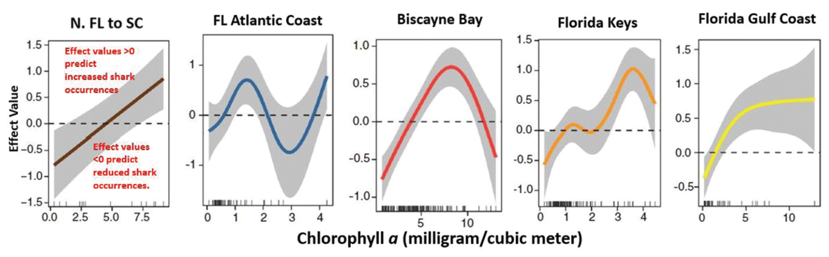
Figure 9
These graphs show the effect of Chlorophyll a on shark detections in each of five study regions. The concentration of Chl a significantly affected the number of days bull sharks were detected at each of the locations.
Student investigations lead to the conclusion that both SST and Chl a had significant effects on the presence of bull sharks in all regions investigated and that shifts in these likely serve as cues to initiate movement related to life history events. One of the main conclusions the investigators inferred from the project results was that Biscayne Bay likely plays an important role in the reproductive cycle of bull sharks.
Summary
An overview of three Grade 8–12 lessons developed using authentic data from the US MBON program was presented. Goals for each of the lessons in the Ocean Animals on the Move series include: 1) Lesson 1—Identifying what can be learned from ocean animal tracking data and simulating field work that requires tracking an animal using active and passive acoustic telemetry; 2) Lesson 2—Recognizing the different types of tags available and determining the appropriate one to use based on the research question; and 3) Lesson 3—Gaining skills in data analysis by investigating the movement patterns of tagged bull sharks and determining potential driving factors to explain the observed patterns. Combined, the lessons teach students about the method, technology and applications of acoustic telemetry. The importance of good data stewardship practices and an understanding that the ocean is a vast, interconnected system of species, habitats and ecosystems that rely on one another for balance, resilience and adaptation are important components of the lessons.
Acknowledgements
Artwork is the original creation of Lori Anzalone, Anzalone & Alvarez Studios. The authors thank Dr. Laura H. McDonnell, Woods Hole Oceanographic Institution, and Dr. Neil Hammerschlag, Atlantic Shark Expeditions, for their contributions to the research data used in these lessons.
Competing Interests
The authors have no competing interests to declare.
Author Contributions
All authors contributed to the conception, writing and reviewing of this manuscript and have approved the submission.
Author Information
Chris Simoniello is a Research Scientist at Texas A&M University and the Outreach and Education Manager for the GCOOS Regional Association. Her work is focused on enabling the use of information about the Gulf’s coastal and open ocean waters to benefit people, ecosystems and the economy. She is committed to creating dynamic mechanisms to nurture innovation and the scientific processes critical to better understanding our world and provide an adventurous call to action for our future ocean leaders.
Mitchell J. Rider is a Postdoctoral Research Associate with the Cooperative Institute of Marine and Atmospheric Studies at the University of Miami. His work focuses on the development of species distribution models for several sea turtle species across the Southeastern United States. He is dedicated to furthering our knowledge on the movement ecology of sea turtles in the region especially with respect to potential interactions with anthropogenic activities.
Mathew Biddle works for the U.S. Integrated Ocean Observing System program office as a data management analyst and has more than 15 years of experience in oceanographic data management. Prior to IOOS, Matt worked with the Biological and Chemical Oceanography Data Management Office at the Woods Hole Oceanographic Institution as a data manager and administrator of their ERDDAP. Before that, he worked with the NOAA National Centers for Environmental Information cataloging, archiving, writing metadata, and making oceanographic data publicly available.
Grant Craig is a program coordinator for GCOOS, one of 11 regions of the US Integrated Ocean Observing System. He has more than 25 years of experience working as an educator, resource manager, and project coordinator focused on the Gulf with an overarching theme of delivering scientific information to non-scientific audiences. His current work focuses on engaging with partners, communities and elected officials to develop and promote data products that benefit regional stakeholders.
Felimon Gayanilo has decades of experience in system design and development in a multicultural, multi-disciplinary and international setting and is presently the Information Systems Architect and Enterprise IT Technologist at Texas A&M University-Corpus Christi. With a background in ecological modeling and fisheries, he is now focused on the collection, curation and distribution of metocean data, serving as point person since 2008 for all in situ observing assets of GCOOS.