
1. Introduction
The fundamental challenge in osteoporosis treatment is understanding the nature of the remodeling process. Here, the fundamental approach to analyzing the phenomenon itself is to describe the interactions between cells and the ways in which information exchange is organized through control signals, typically associated with the secretion of appropriate enzymes and molecules. This creates a balance within the system that leads to maintaining homeostasis, i.e., stimulating the appropriate cells to ensure the formation of the proper trabecular bone structure [1–3]. Understanding and determining the correctness or adequacy of trabecular bone structure in the context of mechanical loads cannot be overlooked. From this perspective, it becomes crucial to consider the actual, spatial bone structure in theoretical studies as a response to the need to transfer external loads [4]. Therefore, the need arises to build research and simulation models that can link biochemical factors and cellular activity with the developing spatial bone structure. It should be noted that this is also related to the way in which the bone structure is loaded. This is highly variable over time, which, from the perspective of simulating the remodeling phenomenon to ensure homeostasis, poses further challenges for numerical models [5–8]. This article presents an approach that allows for the construction of numerical models for simulating the remodeling phenomenon of trabecular bone. This should enable “in silico” studies of the response of the entire bone remodeling system to pharmacological effects under variable external loads. This will require not only incorporating many already known observations but also generalizing the concept of homeostasis using principles known from structural optimization.
2. Materials and methods
2.1. Homeostasis – the essence of remodeling process
Homeostasis, understood as the stimulation of appropriate cells that ensures the formation of the proper structure of trabecular bone, is often described solely as a biochemical system, with mechanical stimulation being one of the factors influencing the system’s functioning. Such a description is often limited to processes occurring within a single basic multicellular unit (BMU) [1]. However, when one looks at the entire process from a broader perspective, one can see that the true goal is to ensure the proper behavior of the bone structure under load, and then homeostasis can be defined somewhat differently. This approach underpinned the idea of viewing the entire process through an engineer’s eyes, as Wolff [9] did two centuries ago, followed by Frost [10], Carter [11], Huiskes et al. [6,7], and many others at the end of the last century. They all observed the rate of trabecular bone growth understood as the observed increase or loss of tissue on the surface of the trabecular bone. A growth value of zero corresponds to a state of homeostasis. The fundamental observation, based on knowledge from biology and medicine, is the dependence of the bone remodeling process on mechanical stimulation. Various studies use different measures of this stimulation. Opinions on this topic remain divided to this day. Huiskes used strain energy density (SED), but in his article [12], he emphasized that he made this choice by chance and that other solutions are possible. In any case, considering the entire structure, one can identify a local degree of stimulation resulting from the external load system. In this perspective, it is necessary to define homeostasis not only locally, as a description of the system’s behavior in relation to a single BMU, but globally, in relation to the mechanical load experienced by the entire organism. Only then it is possible to obtain an appropriate model, allowing for research and simulations reflecting the influence of all significant factors related to the formation of the proper (or improper) spatial structure of trabecular bone. Structural spatiality is not only a term strictly related to mechanical engineering; in the context of trabecular bone, it also reflects two characteristics of the entire remodeling phenomenon, namely:
− the aforementioned sensitivity to mechanical loading, which can only be assessed correctly when the actual form of the loaded structure, i.e., the actual trabecular network, is used for assessment.
− the specificity of the trabecular bone remodeling process, which can only occur on the surface of the trabecular bone due to blood access, and therefore the cells responsible for the remodeling process.
Taking this into account, we can now formulate a description of the remodeling process in relation to the actual spatial structure. Since the phenomenon occurs on the surface of trabecular bone, the model must address changes (tissue growth or loss) occurring on the surface. Hence, the modeling requires spatial models, representing the actual structure of the trabecular network. Although this is significantly more complex than continuous models, it has highly desirable properties for research applications, enabling the assessment of the emerging structure in terms of its strength under various loading conditions. In this sense, such a geometrical description of trabecular bone remodeling can now be considered in the context of its mechanical structure and its resistance to mechanical loads. The similarity of bone structures to solutions to structural optimization problems has, of course, long been recognized [13–15]. However, the possibility of using results from structural optimization in the analysis of bone remodeling is a new idea. Theoretical results will now be presented, allowing for analyzing bone remodeling as a process leading to the creation of a structure with the highest stiffness.
2.2. Homeostasis vs stiffest design – the role of “lazy zone”
Let’s begin by defining the task of finding structures with the highest stiffness. This is a fundamental problem in the design of mechanical structures. Engineers strive to shape the loaded structure so that the assumed loads can be transferred with the minimum possible material volume. The energy stored in the body as a result of external forces should be as low as possible, thus ensuring the structure’s stiffness is as high as possible.
On the one hand, it is important that the reduced stresses caused by the load do not exceed the permissible value for a given material, but on the other hand, it is equally as important that there are no areas in the structure where there is no energy stored, and therefore, the material is not used well. To describe this situation properly, we need to look at the trabecular bone as a spatial structure. This approach will us allow to refer to the principles of structural optimization, in which the objective is to find the optimal distribution of material in three-dimensional space. This is a significant difference from defining structure by its density. Now, the spatial distribution of material with a boundary in the form of bone tissue surface will be considered.
The goal is to minimize the strain energy functional, i.e., the work done on the body in the form of an integral over the region Γ1, where the forces ‘t’ are applied and the strain ‘u’ is obtained, Γ0 is part of the boundary with the Dirichlet condition, and Γv is part of the boundary subjected to modification, as depicted in Figure 1. Since the problem of the stiffest design (compliance minimization) has no solution without additional assumptions, usually the volume of the material in the design domain is limited. The Lagrange equation can be written as follows:
The condition for the optimal structure can be written as follows [16]:The relationship between the Lagrange multiplier and volume constraint exists and was described in a number of papers concerning topology optimization methods [13,17,18]. The assumption of the limit of the available material V o in the Ω domain turns out to be identical to the assumption of the constant, specified value of the Lagrange multiplier λ on the surface (the detailed discussion of this result is presented in [13,19]). It should be emphasized that, based on the results presented in these works, the principle of minimizing energy in volume is replaced by energy equalization on the surface of the structure.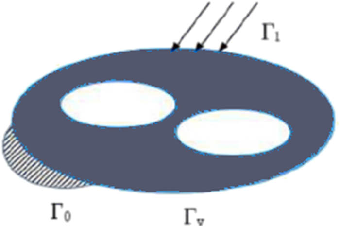
Figure 1
The stiffest design problem description: t applied forces, u displacement, Ω the domain of the elasticity system, Γ 0 part of the boundary with Dirichlet condition, Γ 1 part of the boundary loaded by traction forces, and Γ v part of the boundary subjected to modification.
Thus, the condition for the best spatial shape of the desired structure can be formulated as follows: the SED on the structure’s surface should be constant. But this is precisely what Huiskes intuitively assumed in relation to the trabecular bone remodeling phenomenon. There is a certain value of energy density on the structure’s surface that corresponds to the minimum energy in its entire volume. This is the value of homeostasis. The remodeling process therefore leads to a change in local configuration that will increase (removing material) or decrease (adding material) the energy density on the structure’s surface. Equalizing the energy density across the entire structure’s surface will consequently produce a global effect in the form of a structure with the highest stiffness. This, in turn, corresponds to minimizing the mass of the entire structure because the least material is needed when the energy in the entire structure is minimized.
Therefore, the process of the trabecular bone remodeling can be viewed as a structural optimization procedure that can find the best spatial configuration for a given material. However, unlike theoretical examples, the loads on the bone structure are not constant. They may change significantly, and the proper bone structure must respond to such variable loads. And there is another clinical observation, worth mentioning here, namely, the “lazy zone” in the context of bone stimulation measurement. Frost called the “lazy zone” the stimulation close to the homeostatic value because this name was intended to reflect the fact that with small deviations of stimulation from the homeostatic state (SED values on the structure’s surface), neither an increase nor a decrease in tissue volume is observed. This arrangement means that the load change is only partially reflected in the structural change, and in the long term, the entire bone structure retains a memory of the entire load spectrum.
So, the algorithm for trabecular bone remodeling could be described using the term “bone growth rate” and the concept of “lazy zone” as follows:
where GR is the tissue growth rate, E is the SED on the structural surface, λ is the homeostatic value of the mechanical stimulation, λ − s is the lower SED limit of the “lazy zone,” λ + s is the upper SED limit of the “lazy zone.”This allows the continuously remodeled structure to be prepared for various loads without changing the entire remodeling mechanism. Therefore, in the remodeling procedure, there is not a single value of the Lagrange multiplier corresponding to the homeostatic value, but a zone surrounding this value. To build the model, it is necessary to determine two stimulation values – the minimum and the maximum, constituting the boundaries of the lazy zone. Again, this observation is also important in the area of structural optimization, allowing for the optimization problem to be solved for many load cases [17].
2.3. Trabecular bone treatment – new therapy option
Equipped with such a model based on the principles of structural optimization, it is now possible to attempt to interpret the phenomena occurring during the remodeling process. New therapeutic options have recently emerged [20,21]. Until now, osteoporosis drugs have disrupted the entire trabecular bone remodeling process by inhibiting bone resorption [22]. This is an effective solution, but it carries a number of risks, the most significant of which is the accumulation of microcracks in the bone, which are not repaired by the inhibited osteoclasts. A new approach is to block sclerostin, an enzyme produced by osteocytes and directly related to the mechanical loading of the trabecular bone structure. This approach has the advantage of not interfering with the bone tissue replacement process itself, which is still removed, allowing for the elimination of microcracks. But what is most important from the perspective of planning treatment is the ability to directly interpret the presence of sclerostin as a factor influencing the understanding of homeostasis described earlier. In a normal setting, when the bone tissue is healthy, the amount of sclerostin, as a measure of mechanical stimulation, allows for the determination of how local stimulation relates to the “lazy zone.”
On the cellular level, the pathways of the mechanostat model are extremely complicated. But the very important anabolic feedback in bone remodeling, which modulates the Wnt signaling pathway, leads to another state of homeostasis [16]. The Wnt/β-catenin signaling pathway plays a central role in relation to mechanical stimulation. This pathway allows interference with load-dependent regulation. In the signaling pathway, Wnt-Scl-LRP5/6 sclerostin modulates the signaling pathway by interacting with LPR5/6 receptors. By pharmacologically influencing the amount of sclerostin in turn, the entire pathway can be regulated. The amount of sclerostin is therefore correlated with homeostasis, and this pattern reflects the strength properties of the material from which the tissue is composed. The greater the load on the tissue, the lower the amount of sclerostin, and conversely, when the load decreases, the amount of sclerostin increases. The mechanism of action of the new generation of drugs is based on this very observation. By artificially reducing the amount of sclerostin, the “lazy zone” is modified, and this is exactly how Romosozumab works by acting against sclerostin. This results in not only an increased rate of bone formation but also a decreased resorption, which is considered a “double effect” and the reason for the drug’s high effectiveness. A shift in the “lazy zone” position, i.e., homeostasis definition, means that the amount of stimulation recognized by the “system” is different.
2.4. The treatment models based on “lazy zone” definition
We can now attempt to build simulation models using a change in the assumptions of the “lazy zone” position and size. As evidenced by observations, the concept of homeostasis exists, corresponding to a specific level of mechanical stimulation. Interestingly enough, this also applies to other models, as exemplified by Professor Fung’s publications [23,24]. In any case, through the process of remodeling, the body implements the assumption that the evolution of the structure will ensure a spatial form that has an energy density at the surface close to the homeostatic value. The mechanism of action of drugs, which involves changing the amount of sclerostin, effectively leads to a change in the homeostatic SED value on the tissue structural surface. This translates into a shift of the “lazy zone” (in the direction of the lower stimulation):
− the homeostasis point corresponds to the SED value on the structure’s surface is shifted toward lower SED values
− on the side of greater energy in the zone – a lower SED value will be interpreted by the “system” as sufficient to initiate tissue growth,
− on the side of lower energy in the zone – more tissue will remain unremoved despite the low energy value.
And now it is possible to explain the Romosozumab “dual effect” result. Unlike the other pharmaceutics, which increase both formation and resorption, Romosozumab increases formation and decreases resorption, and this observation is called the “dual effect.” In clinical trials, this resulted in a large bone buildup. But the “dual effect” can be explained directly by the “lazy zone” shift, caused by the Romosozumab action against the sclerostin.
However, in structural optimization studies, such a shift in the lazy zone is related to the material and its strength properties [19]. The value of the SED, defined as the homeostasis value, is the value of the Lagrange multiplier in equation (1). This value varies for different materials; that is, for a material with lower strength (e.g., aluminum compared to steel), the Lagrange multiplier will be smaller. This is consistent with engineering intuition – less volume of a higher strength material is needed to transfer the same loads, and this fact was noted in structural optimization studies [18,25].
In Figure 2, the graphical illustration of equation (3) is presented. The horizontal axis of the graph shows the stimulation measured by the SED value on the surface of the tissue structure. The vertical axis shows the “bone growth rate,” where the value zero corresponds to the inside of the “lazy zone.”
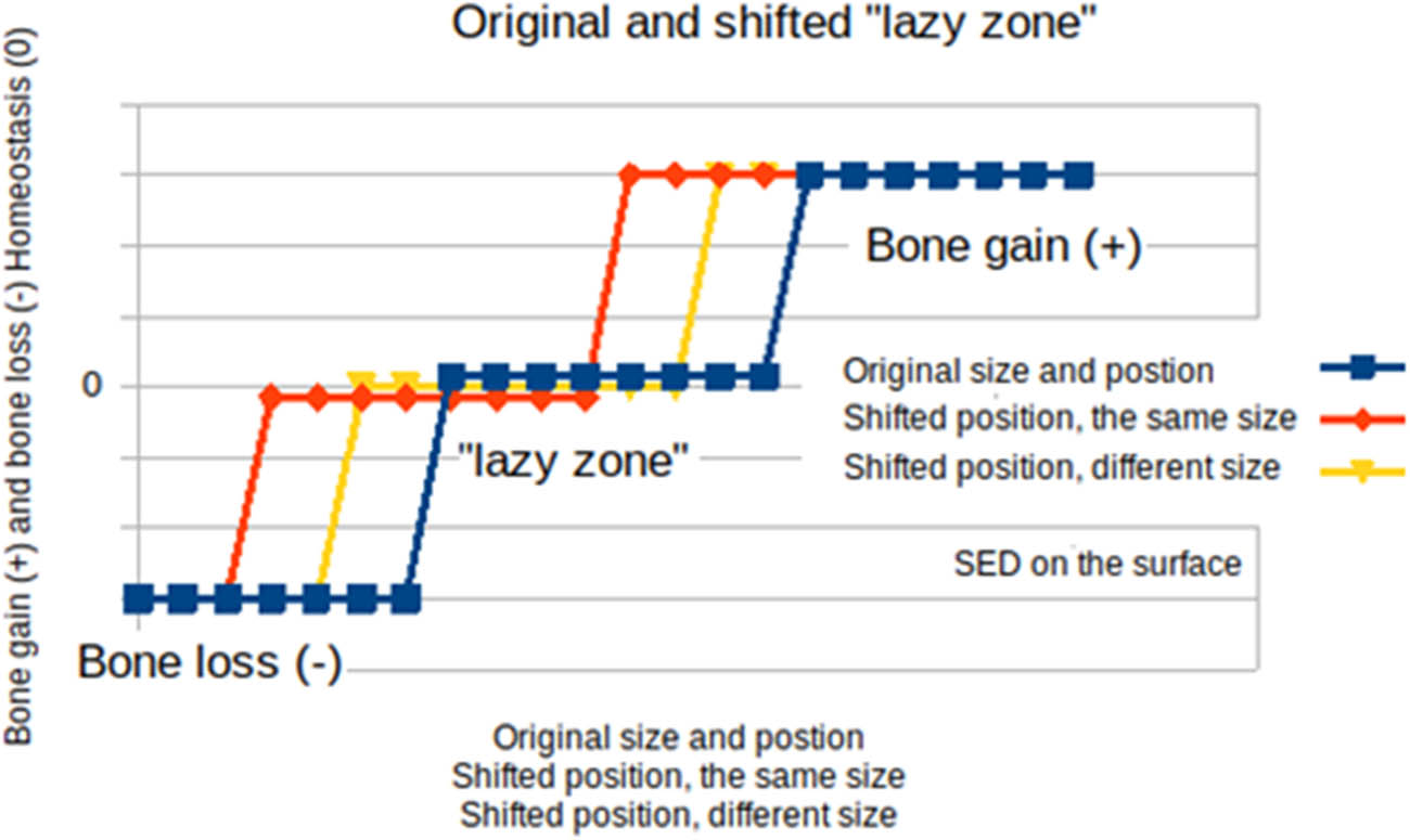
Figure 2
“Lazy zone” size and position – blue: the starting configuration, red: shifted position of the zone with the same size, yellow: shifted position and different size of the lazy zone.
In Figure 2, three different definitions of the zone corresponding to different stimulation values considered homeostasis are presented. The blue color indicates the original position of the zone, the red color indicates the shift, and the yellow color indicates the change in both the position of the zone and its size. From an engineering perspective, Romosozumab’s action can be defined as the adoption of a different homeostasis point, corresponding to different strength properties of the material from which the trabecular bone tissue is composed. However, the entire process follows the same principles, achieving the highest possible stiffness.
3. Results
3.1. Numerical examples of possible bone treatment models
However, the question arises as to how one could assess how the zone should be defined in order to achieve the desired effect in the form of the best use of the material. Here, the structural optimization principles can be used as guidelines for trabecular bone treatment models.
The remodeling process aimed at achieving homeostasis means, according to equation (1), minimization of energy, and therefore, the result is the stiffest design in the sense of structural optimization. If we assume in turn that striving to achieve homeostasis is the goal of the remodeling process, then tests of the proper position of the postponement zone can be carried out for known solutions of tasks in the area of structural optimization. For illustration, one of the examples from the work [26] – “Exact analytical theory of topology optimization with some pre-existing members or elements” was chosen. Pre-existing members, i.e., a fragment of the structure is always preserved and is not removed during the optimization procedure (nondesign area), is important here. It is important to observe changes even when a significant portion, or even the entire analyzed area, is outside the zone. Otherwise, material removal, resulting in a disconnection between the areas where the boundary condition is defined and the loaded areas, would make it impossible to conduct simulations using the structural analysis. The model used for the calculations is a three-dimensional structure with a virtual evolution of the structure’s surface position – details can be found in the previous studies [13,17]. Figure 3 shows the numerical example: scheme of the topology design problem with a nondesign area. The tests were carried out with different positions and “lazy zone” sizes. Material properties were assumed for the aluminum: Young modulus 7 × 10¹⁰ Pa and Poisson ratio 0.3. The calculations started by defining the “lazy zone” in the SED range 3.20 × 10⁴–2.00 × 10⁵ Pa (which corresponds to blue curve on Figure 2), then the zone was moved to different positions at the SED range of 8.00 × 10³–1.28 × 10⁵ Pa (which corresponds to red curve shown in Figure 2), and then, it was moved again, but its size was also changed in the SED range of 2.45 × 10⁴–8.45 × 10⁴ (which corresponds to yellow curve in Figure 2).
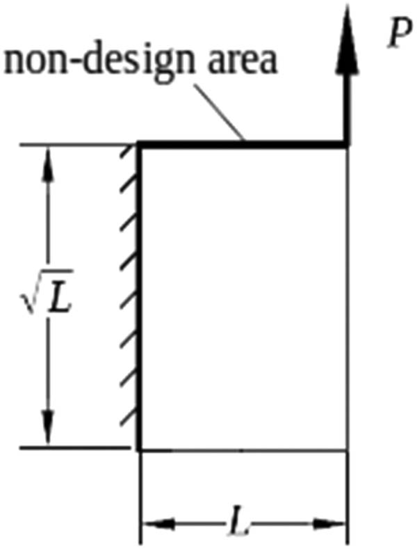
Figure 3
The numerical example: scheme of the topology design problem with a nondesign area – L = 50 mm, P = 1,000 N.
3.2. Structural evolution calculations
The Cosmoprojector system was used for the calculations – details of the numerical implementation can be found in the previous studies [27,28]. This is a system dedicated to the simulation of trabecular bone remodeling. The structure model is three dimensional, so to compare the results with 2D solutions, it was necessary to create a starting configuration in the form of a quasi-2D model. The model’s shape corresponds to the example shown in Figure 3 and the third dimension, i.e., thickness was 5 mm. The force value P = 1,000 N was assumed. The calculations were carried out using the FrontISTR system [27] – Tetra10 tetrahedral type elements were used.
Figure 4 shows the final configurations obtained for different assumptions regarding the “lazy zone.” The final configuration means a situation where the entire surface of the structure is within the “lazy zone,” i.e., there are no areas on the surface for which SED is smaller or larger than the zone range. The result presented in Figure 4 can be interpreted as an illustration of the effect of drugs on the remodeling process. The configuration presented in Figure 4c is the initial state in which the range of the “lazy zone” results in a configuration with a relatively small amount of material. Now let’s assume that the amount of sclerostin has been reduced due to the action of pharmacological agents. This corresponds to a situation in which, despite the lack of mechanical stimulation, the level of stimulation recognized by the “system” is different and an increased amount of tissue will be observed. This is exactly what happened after the “lazy zone” shift, and in Figure 4a, a much larger amount of material can be observed despite exactly the same stimulation level – neither the properties of the material nor the geometric configuration nor the loading force changed. Figure 4c shows yet another configuration, where the zone has been moved, but its size has also been changed. If we can now relate the quantity, the method of application, and the reaction of the entire system to the applied treatment, it will be possible to determine all these parameters in “in silico” studies. Having the results of numerical simulations, it will be possible to compare them with known results from the area of structural optimization. In the presented example, the closest to the known solution (see [26]) is shown in Figure 4b.
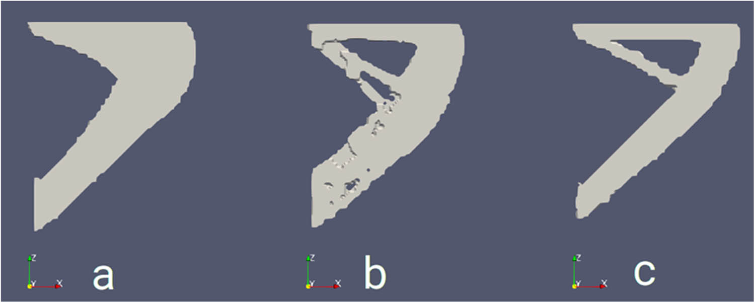
Figure 4
The numerical example, solutions: a – solution for the “lazy zone” range 8.00 × 10³–1.28 × 10⁵ Pa (which corresponds to red curve shown in Figure 2), b – solution for the “lazy zone” range 2.45 × 10⁴–8.45 × 10⁴ Pa (which corresponds to yellow curve shown in Figure 2), solution for the “lazy zone” range 3.20 × 10⁴–2.00 × 10⁵ Pa (which corresponds to blue curve shown in Figure 2).
4. Discussion
The presented results illustrate only a sketch of the idea. A very simple numerical example is forced by the need to compare it with analytical solutions. However, this makes it possible to actually take into account the location of the “lazy zone.” Now, a similar study can be conducted for actual trabecular bone structures by observing the evolution of the spatial structure of trabecular bone for different homeostasis values indicated by the energy density on the surface of the structure. The result presented in Figure 5 can be interpreted as an illustration of the effect of drugs on the remodeling process.
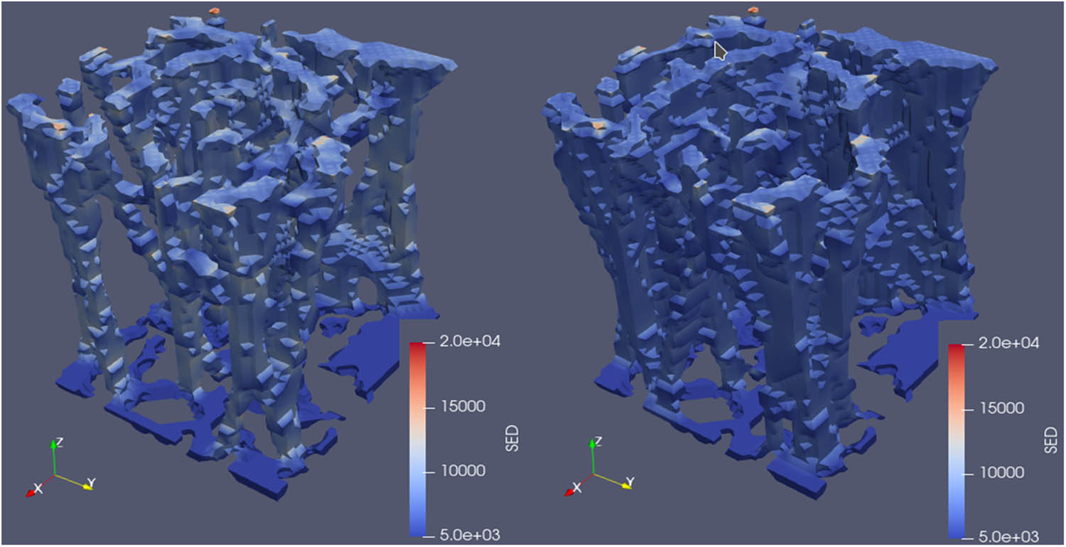
Figure 5
The numerical example, solutions: left – solution for the original “lazy zone” position and range (which corresponds to the blue curve in Figure 2), right – solution for the shifted “lazy zone” position and range (which corresponds to the red curve in Figure 2.).
Further research is necessary – of particular interest is the relationship between surface energy density and material strength, and therefore the strength hypothesis. However, an appropriate hypothesis would first need to be formulated. In the context of the action of pharmaceuticals related to sclerostin, the location of the “lazy zone” can be treated as a result of their action. It can therefore be expected that appropriate studies in the area of structural optimization can significantly contribute to determining the desired targets of action of pharmaceuticals. What is immediately noticeable is the dependence of the amount of material on the location of the “lazy zone.” But you can also see the different topologies of the solutions obtained. This aspect of the matter is of decisive importance when assessing the properties of trabecular bone tissue. But the assessment must concern the entire spatial shape, and this in turn is related to the strength properties of the material. Too large a “lazy zone” or too strong a shift will have an unfavorable effect on the entire structure, as microcracks will remain and the position of the zone will not correspond to the material properties.
The highest priority in this context is to correlate material properties with the Lagrange multiplier value. This problem is also extremely important from the point of view of structural optimization. Therefore, further research in interdisciplinary teams is needed. The basic research problem on the medical side is to determine the strength parameters of bone tissue. This would allow for the construction of a proper model based on the concept of homeostasis, using the “lazy zone” concepts and tools enabling the simulation of larger tissue fragments [28,29]. The team continues to develop software that offers hope for realizing such scenarios. As computational capabilities improve, this goal may become achievable. The presented approach, software, and simulation possibilities are an essential tool for developing treatments for chronic bone diseases, particularly osteoporosis, which is characterized by disruption of the micro-architecture of trabecular bone.
Funding information
Authors state that no funding information.
Author contributions
The author contributed to all aspects of the study, including conceptualization, methodology, analysis, and writing of the manuscript.
Conflict of interest statement
The author states no conflict of interest.