
Table 1
Variables used in the study.
| VARIABLES TYPE | DESCRIPTION – VARIABLE | CODE OF JUSTICE IN NUMBERS** |
|---|---|---|
| Predictor variables | ||
| Actual access to the judiciary |
| casos_novos |
| Potential access to the judiciary |
| mag_por_pop |
| Explanatory variables | ||
| People |
| mag_por_pop |
| f4a | |
| tfauxt | |
| Administrative structure | varas_por_pop | |
| ICTs |
| dinf1 |
| dinf2 | |
| Education |
| escolarizacao |
| analfabetismo | |
| Income |
| gdp |
| Control variables |
| h2 |
| k | |
| gt | |
| agua_canalizada | |
| nasc_vivos | |
| DAÍ | |
| DPI | |
| coef_gini | |
| taxa_mulher | |
| idade_50 | |
| cor_raca_nao_branca | |
| tempo_medio_decisao | |
| f2 |
[i] * Variables transformed through logarithmic transformation (Box & Cox, 1964), ** (CNJ, 2021).
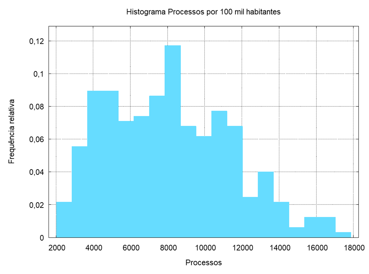
Figure 1
Histogram of the dependent variable (processes per 100 thousand inhabitants).
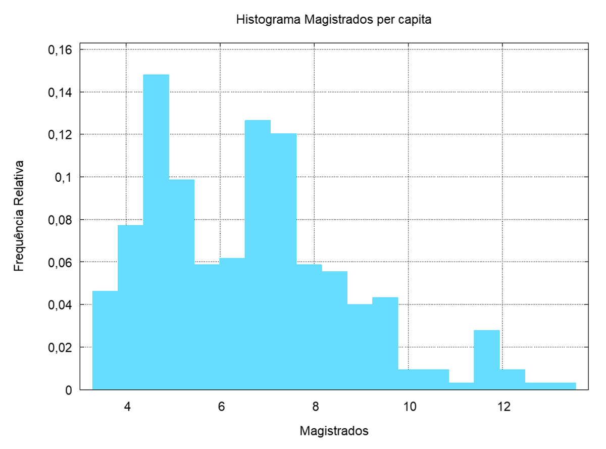
Figure 2
Histogram of the dependent variable (magistrates per capita).
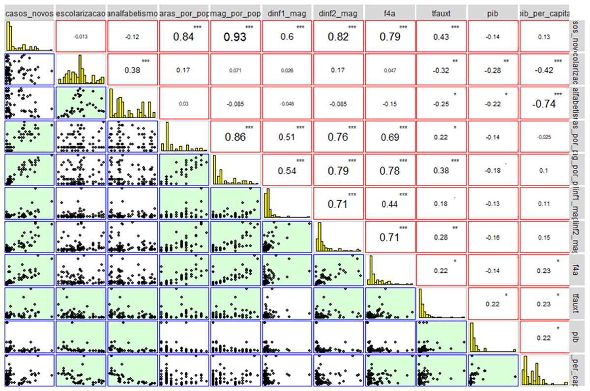
Figure 3
Distribution of correlations and bivariate analyses.
Table 2
Multiple linear regression results.
| MODELS | ||||
|---|---|---|---|---|
| Y1 | Y2 | |||
| (1) | (2) | (3) | (4) | |
| J/POP | 43,847,012.0000*** (8,979,453.0000) | 45,585,121.0000*** (7,659,770.0000) | –12,400.0000 (13,099.4700) | |
| Staff | 14.6482** (6.7953) | 14.5351** (6.1299) | 0.0443*** (0.0070) | 0.0412*** (0.0057) |
| OW | 0.0633 (0.1040) | –0.0002 (0.0001) | –0.0003*** (0.0001) | |
| Courtrooms | 553,252.2000 (10,763,276.0000) | –13,332.8000 (13,449.4100) | –22,784.0600** (11,109.5800) | |
| ICT1 | 0.0011 (0.0010) | 0.0000 (0.000001) | ||
| ICT2 | 0.0027*** (0.0009) | 0.0030*** (0.0006) | 0.000001 (0.000001) | 0.000001 (0.000001) |
| EDU | –499.8882** (202.3117) | –363.9731** (146.5130) | –0.2434 (0.2645) | |
| ILLT | 65.3607 (63.8436) | 0.1174 (0.0797) | ||
| GDP | –0.0000** (0.0000) | –0.0000* (0.0000) | –0.0000* (0.0000) | –0.0000* (0.0000) |
| POP | 4.0934* (2.3854) | 3.1541 (2.1547) | 0.0048 (0.0030) | 0.0037 (0.0025) |
| W | 0.0907** (0.0355) | 0.0973*** (0.0338) | –0.00004 (0.00005) | |
| TCE | –0.0000*** (0.0000) | –0.0000*** (0.0000) | –0.0000*** (0.0000) | –0.0000*** (0.0000) |
| RHP | 21,238.1100** (9,206.0110) | 11,540.2800** (5,138.1140) | 31.0433*** (11.4247) | 19.4942*** (4.1361) |
| LB | 16,492.2100* (9,447.0280) | 16,066.5000* (8,514.2040) | –1.5280 (12.1620) | |
| HAD | 177.3723 (114.1018) | 179.3684* (105.4078) | –0.0693 (0.1460) | |
| WAD | –518.1639* (260.3605) | –328.9689 (221.8510) | –0.1604 (0.3369) | |
| Gini | –8,722.1500 (9,518.4850) | –15.4828 (11.9064) | ||
| RW | 13,208.1000 (19,284.3400) | –30.8830 (24.0630) | ||
| MA | –24,855.6500** (11,756.2100) | –13,261.4100 (8,243.2560) | –12.8704 (15.2095) | |
| NWP | –4,494.3790* (2,303.2390) | –1,765.5630 (1,312.6850) | –4.0666 (2.9395) | |
| APT | –0.3572 (0.6226) | 0.0006 (0.0008) | ||
| J | –161.6616* (95.7380) | –183.6477** (88.2937) | ||
| New Cases | –0.0003* (0.0002) | –0.0004*** (0.0001) | ||
| Constant | –9,794.7120 (12,584.2000) | 4,708.3700 (8,575.5490) | –5.9164 (15.8970) | –11.5679*** (3.8664) |
| Observation | 89 | 89 | 89 | 89 |
| R2 | 0.9486 | 0.9448 | 0.8964 | 0.8855 |
| Adjusted R2 | 0.9315 | 0.9334 | 0.8619 | 0.8725 |
| RSE | 946.0964 (df = 66) | 932.8215 (df = 73) | 1.1910 (df = 66) | 1.1443 (df = 79) |
| F-statistic | 55.4003*** (df = 22; 66) | 83.2423*** (df = 15; 73) | 25.9567*** (df = 22; 66) | 67.8899*** (df = 9; 79) |
[i] Notes: Y1 and Y2 are the first and second dependent variables, respectively. R² (coefficient of determination) represents the proportion of variance in the dependent variable explained by the model; values closer to 1 indicate greater explanatory power. Adjusted R² accounts for the number of predictors included, reducing the risk of overestimating model fit when irrelevant variables are added. RSE is an acronym for Residual Standard Error, which measures the average deviation of residuals from the regression line, with smaller values indicating better model fit. The F-statistics evaluate whether the model as a whole significantly explains variation in the dependent variable; higher values with statistical significance (***) suggest that the predictors jointly contribute to the model. (df) indicates degrees of freedom associated with the model. Significance levels: *p < 0.1; **p < 0.05; ***p < 0.01.
Table 3
Summary of hypotheses and their results (potential and effective access).
| HYPOTHESIS | DESCRIPTION | RESULT |
|---|---|---|
| H1 | The number of judges positively impacts actual access to the judiciary. |
|
| H2 | The number of public servants positively impacts the potential access to the Judiciary. |
|
| H2B | The number of public servants positively impacts actual access to the judiciary. |
|
| H3 | The number of outsourced civil servants positively impacts the potential access to the Judiciary. |
|
| H3B | The number of outsourced civil servants positively impacts actual access to the judiciary. |
|
| H4 | The number of judicial units positively impacts the potential access to the judiciary. |
|
| H4B | The number of judicial units positively impacts the actual access to the judiciary. |
|
| H5 | Investment in technology positively impacts potential access to the judiciary. |
|
| H5B | Investment in technology positively impacts actual access to the Judiciary. |
|
| H6 | The cost of technology positively impacts the potential access to the judiciary. |
|
| H6B | The cost of technology positively impacts actual access to the Judiciary. |
|
| H7 | The educational attainment rate positively impacts the potential access to the Judiciary. |
|
| H7B | The educational attainment rate positively impacts actual access to the judiciary. |
|
| H8 | The illiteracy rate negatively impacts the potential access to the judiciary. |
|
| H8B | The illiteracy rate negatively impacts actual access to the judiciary. |
|
| H9 | Population income positively impacts potential access to the judiciary. |
|
| H9B | Population income positively impacts actual access to the judiciary. |
|