
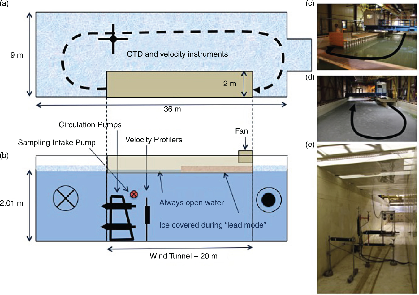
Fig. 1
The CRREL Test Basin set-up for the GAPS Experiment. (a) Plan view diagram. Light blue pattern indicates ice cover water. (b) Section view diagram, showing circulation pumps and location of velocity sensors. Pink shows 96 % ice cover. (c) View looking west across the Test Basin. The wind tunnel is along the left-hand side and the box containing the fan is shown. (d) View looking east across the Test Basin. The end of the wind tunnel is seen on the right. Arrows represent the flow of the water under the ice. (e) A picture looking west down the channel at the wind tunnel ceiling, the velocity sensors and the circulation pumps.
Table 1. Description of the physical properties and results from each of the gas exchange forcing experiments during GAPS
(1−f)Open water
(f)Pump
(Hz)Air temperature
(°C)Water temperature
(°C)U10
(m/s)Cd windv
(m s−1)z (m)vice
(m s−1)keff
(m d−1)k
(m d−1)Std. error in k
1279Convection0.001.000N/R3.0N/R1.4E–030.000.000.000.570.570.342295Current0.760.2440N/R−1.5N/R1.4E–030.030.540.000.251.050.053297Current0.390.6140−3.4−1.4N/R1.0E–040.050.440.000.821.340.014299Current0.390.6160−3.8−1.43.461.4E–030.070.540.010.911.500.155300Current0.390.6120−4.5−1.42.692.0E–040.030.550.010.440.720.056304Current0.210.7960−4.5−1.42.353.0E–040.100.570.011.622.050.097304Current0.210.7940−4.5−1.41.292.8E–030.070.500.010.991.260.038305Current+convection0.210.7940−10.0−1.41.621.0E–040.060.550.011.551.960.029305Current0.210.7940−2.8−1.30.601.6E–010.060.490.011.171.490.0710306Current0.210.7920−2.9−1.31.651.0E–040.030.530.010.360.460.1011309Current0.001.0060N/R−1.21.291.0E–040.100.480.001.491.490.0512310Current+convection0.001.0060−18.0−1.41.291.2E–030.090.470.003.443.440.4113313Current0.910.0960−2.8−1.50.284.0E–040.240.510.000.262.850.2014316Current0.910.0920−6.1−1.41.111.0E–040.070.510.000.131.440.1715320Current+wind0.910.095−3.6−1.46.651.0E–040.030.510.000.333.670.2916323Wind0.910.095−3.4−1.32.437.0E–040.020.510.000.000.020.3417334Current+wind0.960.0460−5.4−1.53.916.0E–040.250.510.000.112.861.3418336Wind0.960.045−3.4−1.57.161.0E–030.020.510.000.030.650.4819339Current+wind0.960.0440−3.5−1.55.673.0E–040.120.510.000.287.652.56
[i] The forcing condition describes whether currents, wind and/or convection were in effect, which relates to the fan and water pump intensity (Hz). The wind speed profile was used to estimate the drag coefficient (C d), assuming a log linear relationship between wind speed and height above the water surface. Using C d and the measured wind speed inside the wind tunnel, we subsequently calculated the 10 m wind speed (U10), using the method described by Mesarchaki et al. (2015). The term v ice is the ice velocity, v is the water current speed; the difference between the two is the water–ice relative velocity (v s) used in the text. The average values of k eff, k and the standard deviation of k. C d, drag coefficient.
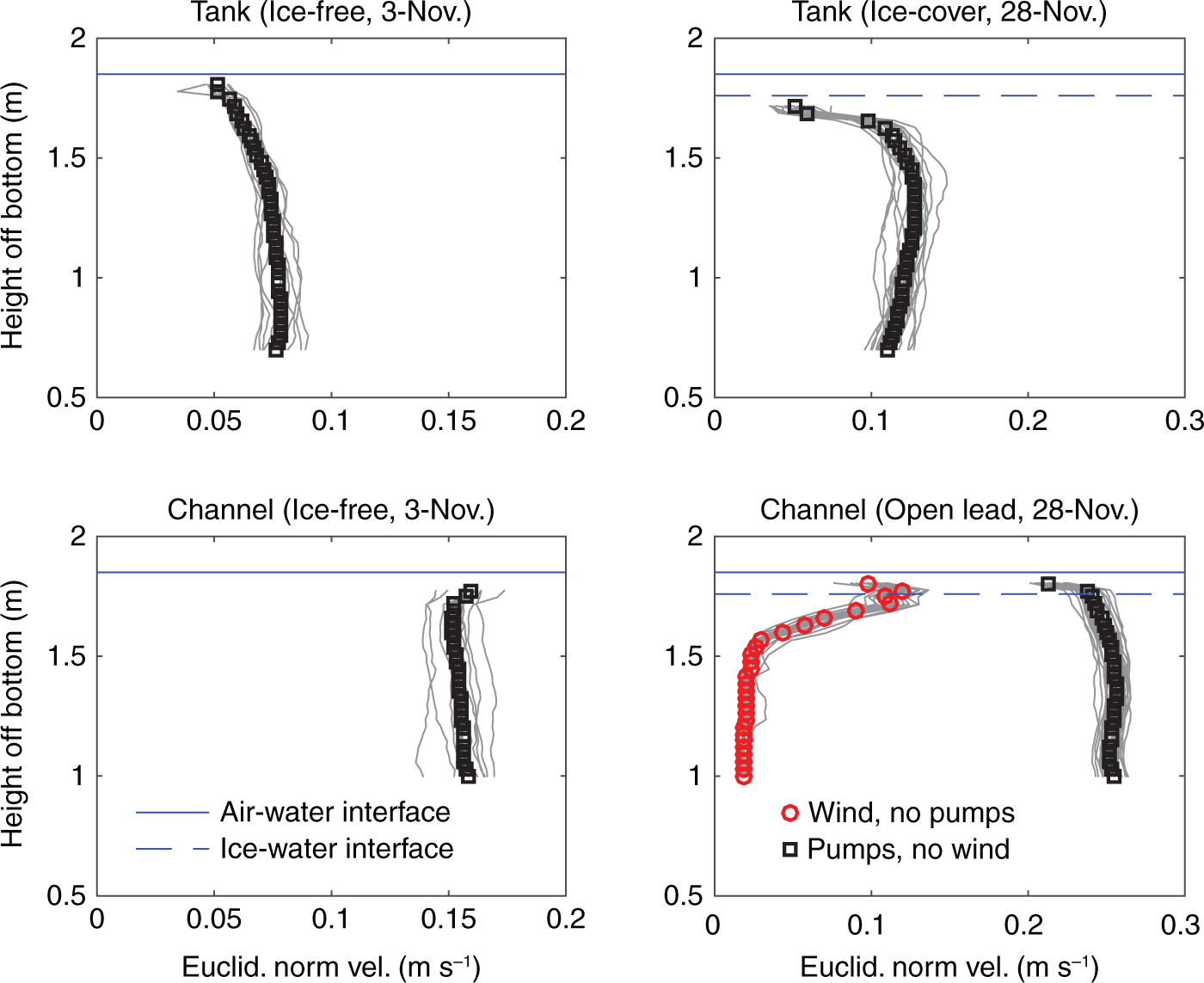
Fig. 2
Profiles of water velocity measured by acoustic Doppler profiler in the ‘channel’ beneath the wind tunnel and in the ‘tank’ outside the wind tunnel. The panels labelled ‘Ice-free’ show velocity during a coincident 12-hour period in the tank and channel with no ice cover. The panels labelled ‘Ice cover’ and ‘Open lead’ (black profiles) show velocity profiles during a coincident 22-hour period. The channel velocity was measured beneath a ‘lead’ opening in the ice, so it was never directly ice covered. The red profile in panel 4 reflects wind forcing with almost no water pump forcing.
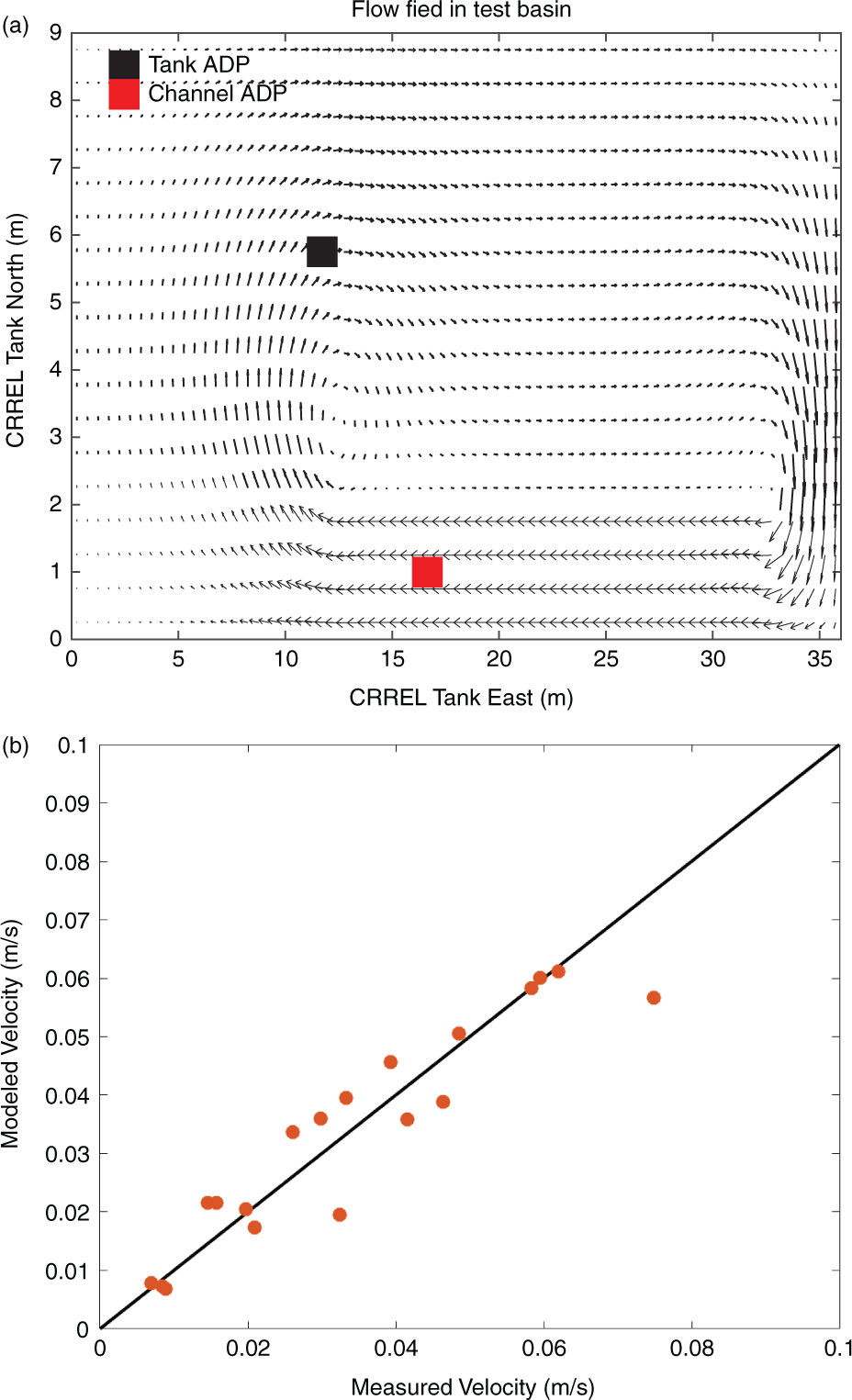
Fig. 3
(Left) Flow field as determined by a finite volume solution to the Boussinesq equations with variable density (Loose et al., 2005). The mean shear velocity (v s) produced in the channel is 0.047 m s−1 in the simulation that is depicted. Right panel, a comparison between measured v s by the Tank ADP and the modelled velocity at that location. Forcing for each simulation was produced using the values of v s that were measured at the Channel ADP location as input, reflecting the action of the circulation pumps.
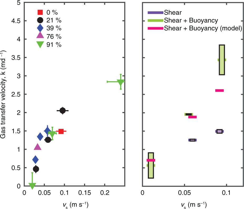
Fig. 4
(Left) Relationship between the water–ice relative velocity (v s) and k for all of the experiments, where v s was the only significant source of turbulence at the air–sea interface. (Right) The gas transfer velocity produced shear + convection (green lines), as compared with the model for gas transfer as a function of TKE dissipation (Zappa et al. 2007) (pink bars). For reference, the k by shear alone (purple bars) has been included at v s=0.06 and 0.09 m s−1 to illustrate the enhancement that results from convection. The shaded black boxes represent the standard error in the estimates of k.
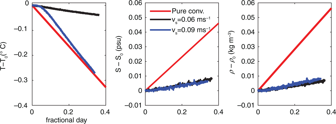
Fig. 5
(Left, middle and right) Temperature, salinity and the resulting density changes during the three convection events where buoyancy losses from the Test Basin were used to induce air–sea gas exchange. The initial T, S conditions for the three events were as follows: Experiment 1, Pure convection: (2.7, 26.4), Experiment 8, v s=0.06: (−1.1, 26.9), Experiment 12, v s=0.09: (−1.44, 26.9).
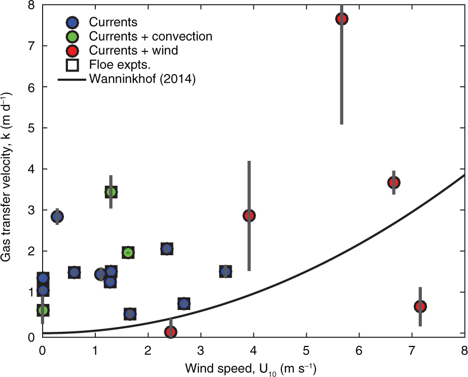
Fig. 6
The gas transfer velocity, k, compared with the average 10 m wind speed in the wind tunnel during the given experiment. The ‘square’ symbols denote estimates during the floe experiments, where open water existed outside the wind tunnel.
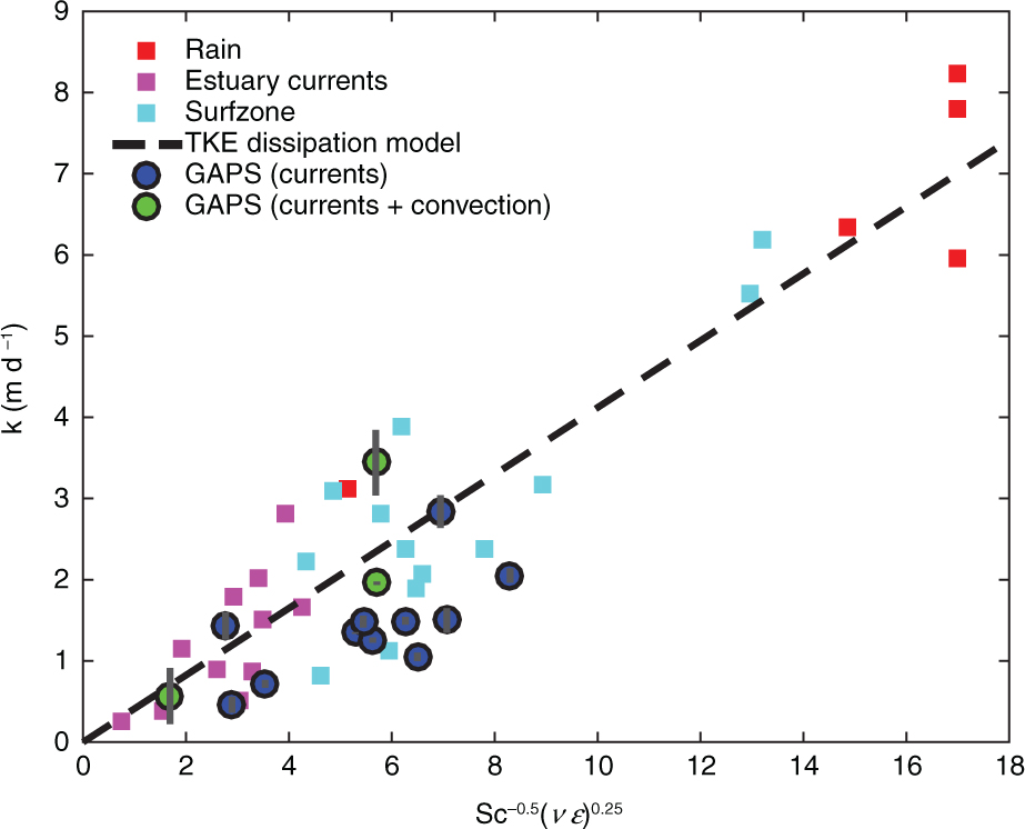
Fig. 7
Scaling between gas transfer velocity (k) and TKE dissipation (ɛ), from Lamont and Scott (1970). The coloured squares originate from Zappa et al. (2007), indicating estimates of gas transfer driven by rain, estuarine tidal processes and surf zone turbulence.