
Table 1. Analytical result on chemical constituents in PM1 (this study)
 (ng m−3)
Avg±SD(µg m−3)
(ng m−3)
Avg±SD(µg m−3) (%)
(%)PM1500113±7210
 1712.5±14.314Cl−32.0±2.320
 8.74.3±5.420
 1212.5±9.214Na0.112.7±2.022K0.111.4±1.122Ca0.114.1±3.722Fe6.252.6±2.010Mg0.10.8±0.710(ng m−3)
As2.120.4±2.810Cd1.3342.2±239.810Co2.080.1±0.510Cr4.13357.8±436.210Cu10.4261.1±152.410Ni2.08179.1±375.910Pb22.928913.2±2874.610Se2.0829.0±38.810V2.08244.1±401.610Zn2.08994.5±3502.910Mn2.0835.3±88.510
[ii] bAdopted and modified after (Mehta et al., 2009).
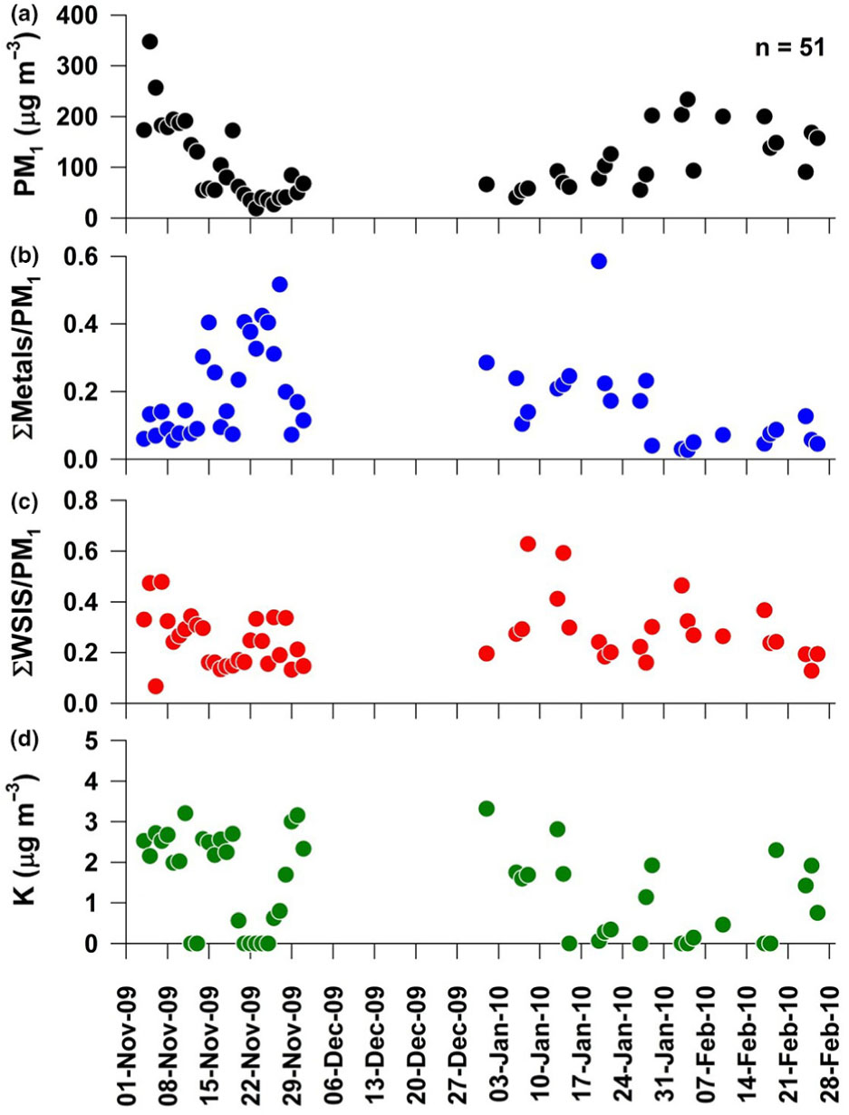
Fig. 1
Temporal variability of: (a) PM1; (b, c) mass fractions of metals and water-soluble inorganic species (WSIS) and (d) K (fine-mode) mass concentration.
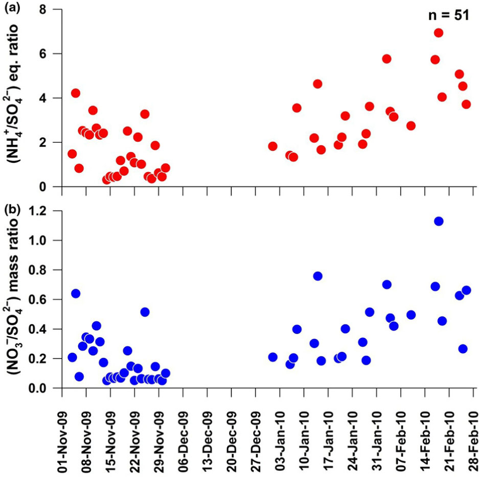
Fig. 2
Temporal variability of: (a) ammonium-to-sulphate equivalent ratio and (b) nitrate-to-sulphate mass ratio.
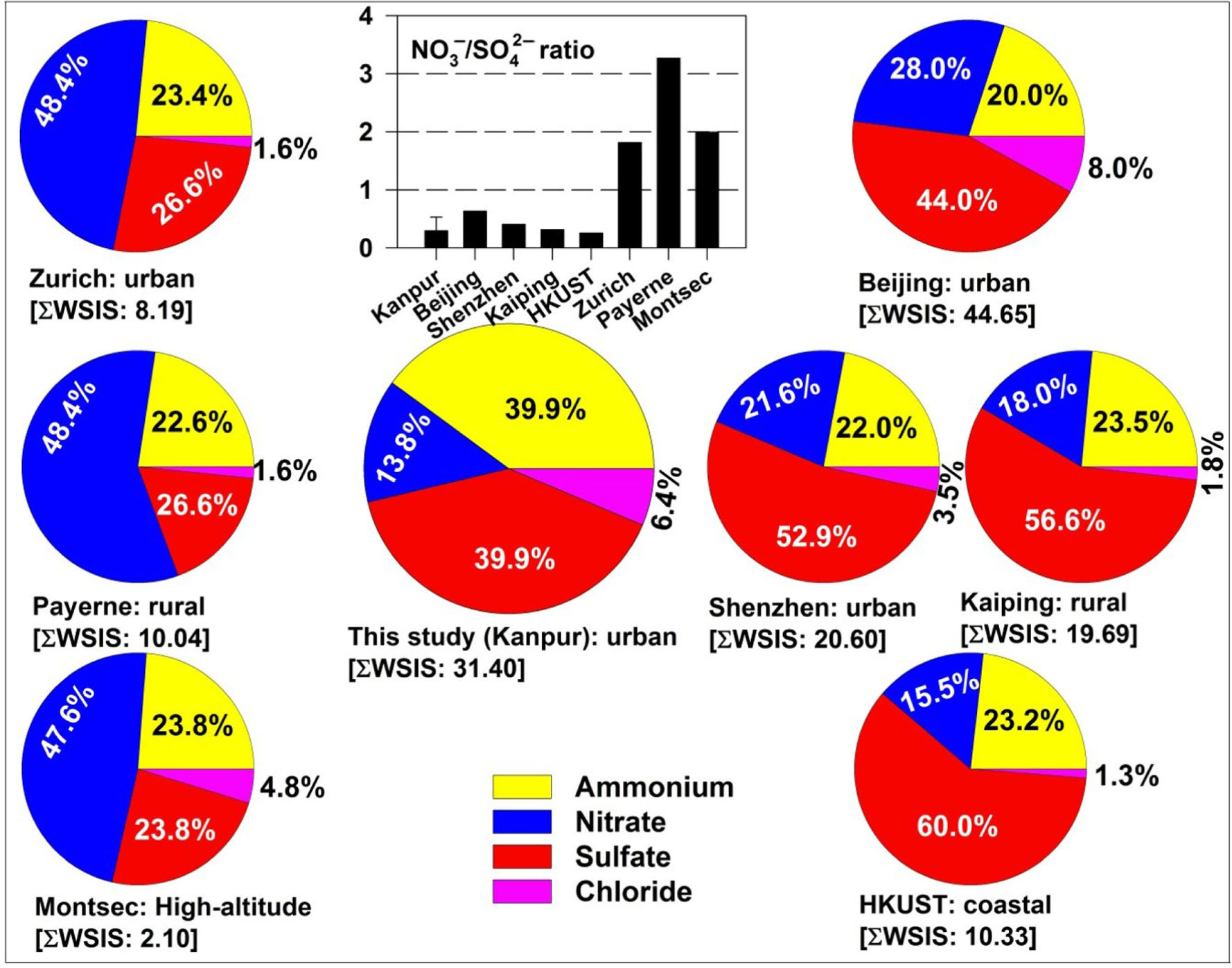
Fig. 3
Spatial variability in chemical composition of WSIS (here SWSIS=
+
+
+ Cl−) in PM1 from some of the urban, rural, coastal and high-altitude locations. Also shown is the nitrate-to-sulphate mass ratio for these locations. Mass concentration of ∑WSIS [given in brackets] is in µg m−3.
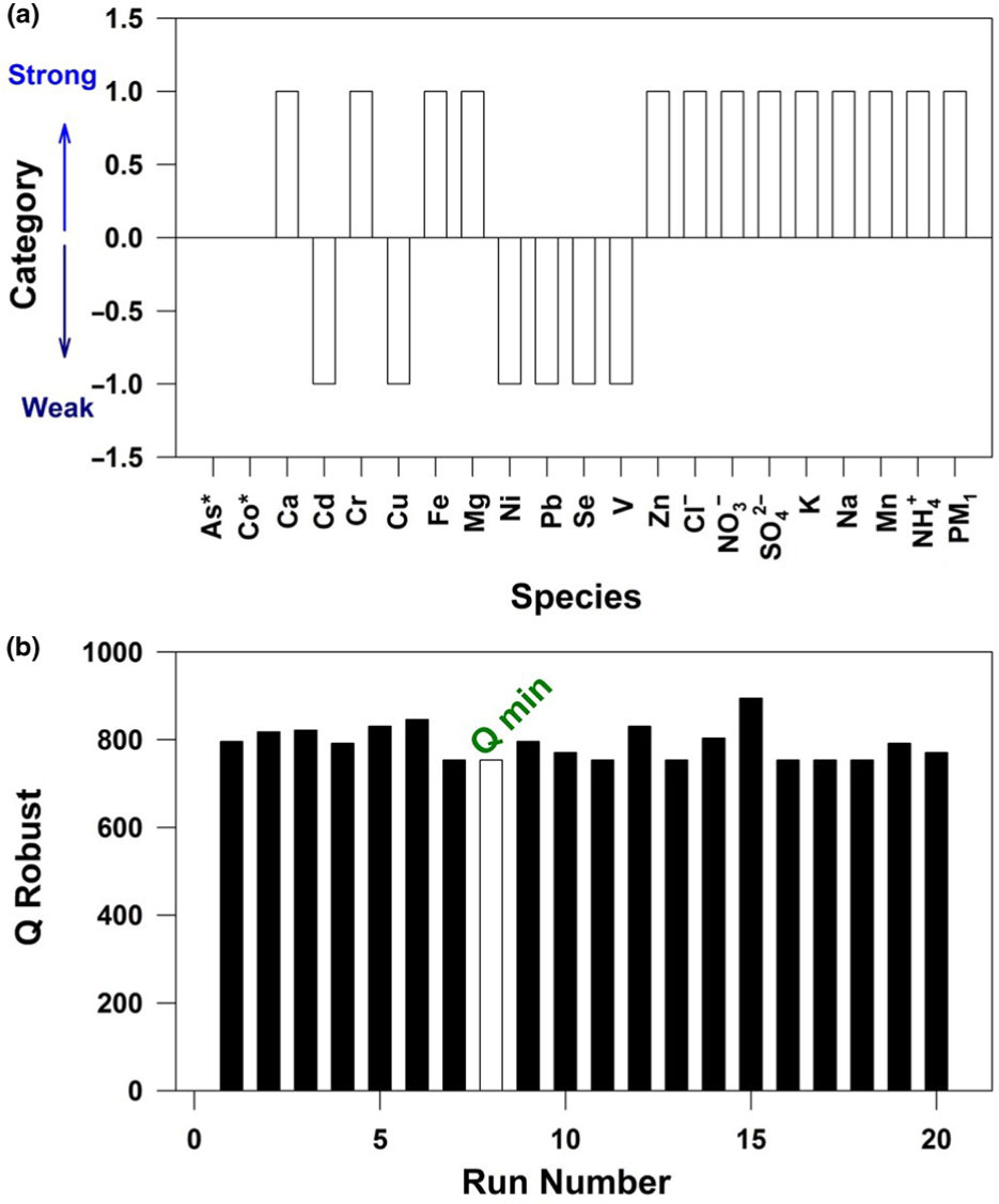
Fig. 4
PMF analysis showing: (a) Species labelled as strong and weak (arbitrary scale on Y-axis) based on residual and regression analyses. Species with asterisk (As and Co) represent the bad species. (b) Variability of Q-Robust as a function of run number.
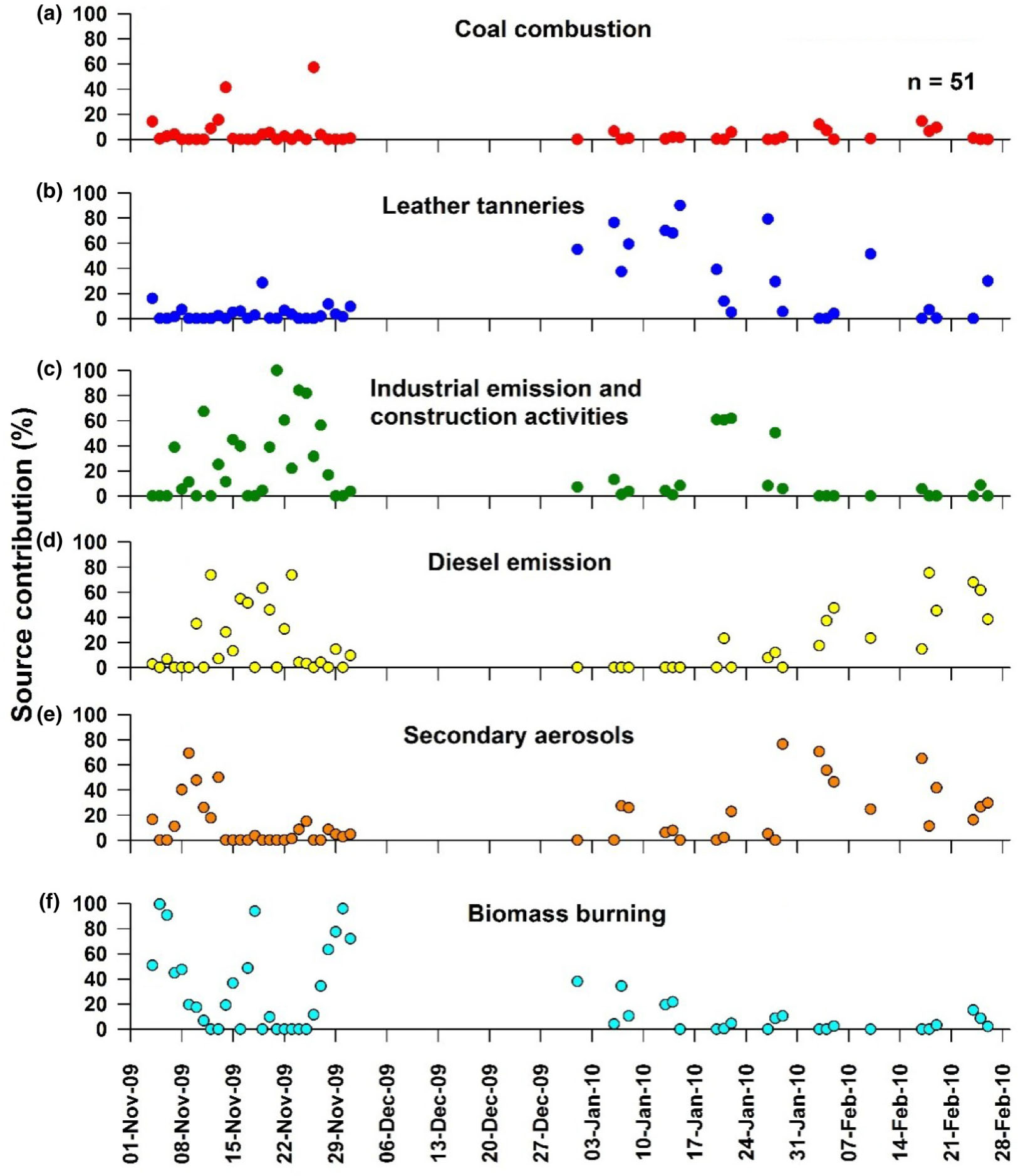
Fig. 5
PMF-based percentage contribution of resolved factors in PM1.
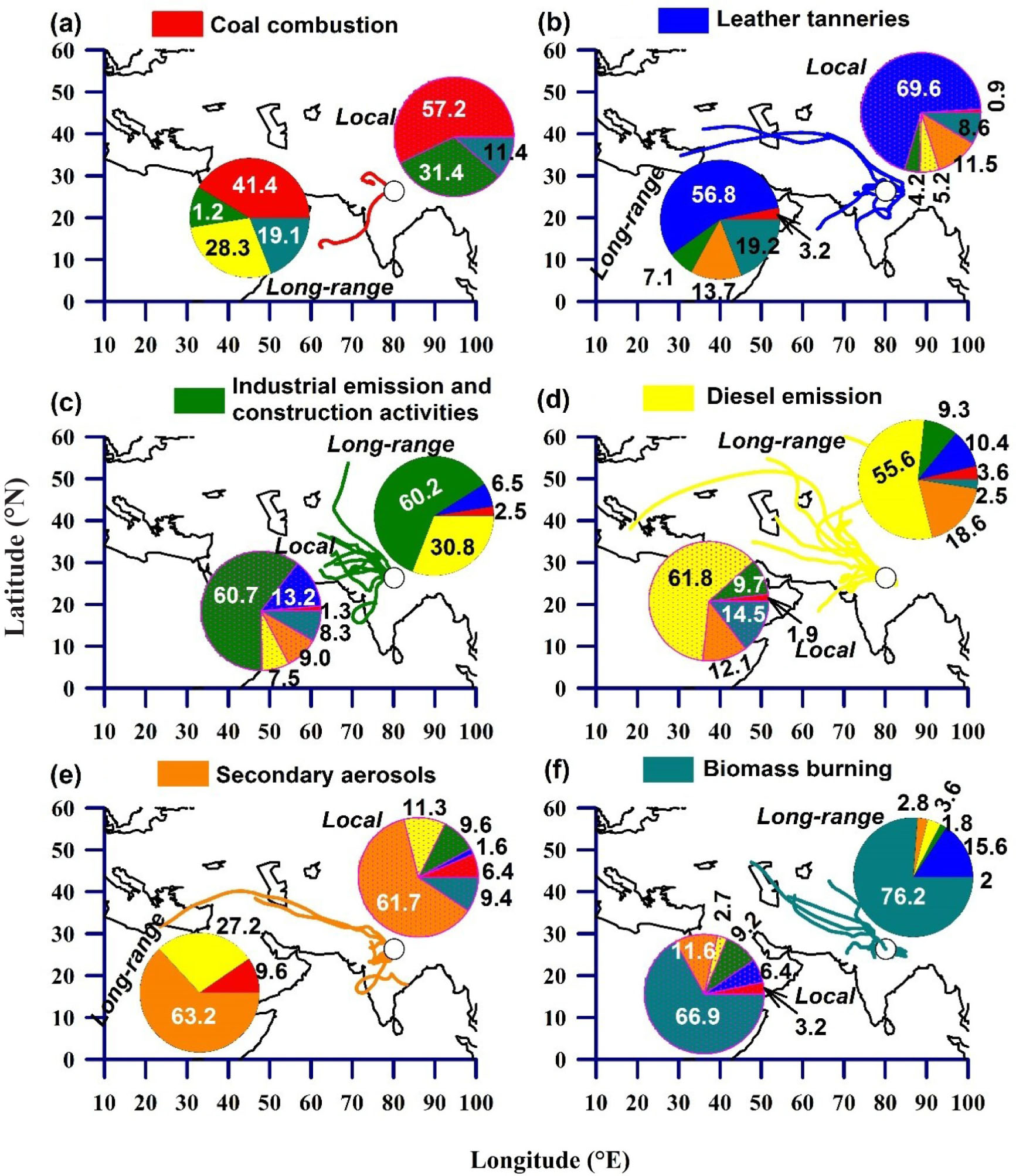
Fig. 6
Percentage contribution of resolved sources in conjunction with air-mass back trajectories (5 d; 1000 m above mean sea level) on sampling days at Kanpur (shown by a circle) shows the predominance of: (a) coal combustion; (b) leather tanneries; (c) industrial emission and construction activities; (d) diesel emission; (e) secondary aerosols and (f) biomass burning emissions.