Chemical characterisation and source apportionment of PM1 during massive loading at an urban location in Indo-Gangetic Plain: impact of local sources and long-range transport

2.1. PM₁ sampling

Sampling location at Kanpur is situated in the central part of the IGP. Kanpur is one of the densely populated and polluted cities in Northern India. IGP experiences extreme weather conditions: harsh summer (April–June; Temp: ~45 °C; wind: 8–10 m/s, SW) and cold winters (December–February; Temp:<5 °C; wind: ~3 m/s, N to NW). Low visibility has been witnessed owing to severe haze and fog events here during wintertime. In this study, PM₁ samples (n=51) have been collected using our own-developed and field-tested low volume air-sampler (calibrated flow rate: 10 LPM) (Chakraborty and Gupta, 2010). Each sample was collected onto pre-conditioned Teflon filters (47 mm diameter). PM₁ sampling has been carried out on the rooftop of a 12 m tall building (Western Lab Extension) in the premises of Indian Institute of Technology (IIT) Kanpur (lat: 26.30°N; long: 80.13°E; 142 m above mean sea-level). Aerosol sampling was carried out continuously for 8–10 h (air filtered: ~5 m³) during the daytime from November 2009 to February 2010. These filters were stored at −19 °C until analysis. PM₁ mass loading has been ascertained gravimetrically on an analytical balance after equilibrating filters (pre- and post-sampling) at about 35 % RH and 25 °C temperature.

2.2. Chemical analysis

For the determination of WSIS ( , , and Cl⁻), aerosol sample was extracted with Milli-Q water (resistivity: 18.2 MΩ cm) using a standardised sonication technique (10 mL×3; 5 min each) and then the particles were allowed for gravity settling. Subsequently, these aqueous extracts were transferred gently in the vials for determination of water-soluble ions on ion-chromatograph (Compact IC 761, Metrohm). A mixture of Na₂CO₃ (3.2 mM) and NaHCO₃ (1.0 mM) was used for the elution of anions, whereas 0.7 mM dipicolinic acid solution with 0.01 % conc. HNO₃ (15.2 N, Seastar; Suprapure, 67–70 % GR grade, Fisher, Leicestershire, UK) has been used for cation. Furthermore, a separate portion of PM₁ sample was treated with 20 mL of conc. HNO₃ (15.2 N, Seastar; Suprapure, 67–70 % GR grade, Fisher, Leicestershire, UK) at ~180 °C on a hot-plate till near dryness for the digestion of trace metals (As, Cd, Co, Cr, Cu, Ni, Pb, Se, V, Zn and Mn) and major elements (Na, K, Ca, Fe and Mg). Subsequently, the final volume was made to 100 mL using Milli-Q water. Then, it was filtered through a 0.22-µm Teflon filter. Quantitative determination of all metals reported herein has been performed on Inductively Coupled Plasma-Optical Emission Spectrometer (ICP-OES; iCAP 6300, Thermo Scientific) (Chakraborty and Gupta, 2010). A five-point calibration (R ²>0.999) on ICP-OES was achieved using a multi-element standard solution (Fluka, 54704). Quality assurance and control pertaining to the data have been assessed in this study based on assessment of several blank filters and repeat analysis. We have processed a total of four blanks in batches along with samples for water-soluble ions and metal analysis (reference is made to Table 1 for method detection limit: MDL). All concentrations of constituents in PM₁ reported herein are blank corrected values (Table 1). Repeat analysis (n=6 for metals and n=5 for ions) of aerosol samples suggest that analytical uncertainty of the measurements is within±6 %.

Table 1. Analytical result on chemical constituents in PM₁ (this study)

Species(ng m⁻³) Avg±SD(µg m⁻³) (%)

---

PM₁500113±72101712.5±14.314Cl⁻32.0±2.3208.74.3±5.4201212.5±9.214Na0.112.7±2.022K0.111.4±1.122Ca0.114.1±3.722Fe6.252.6±2.010Mg0.10.8±0.710(ng m⁻³)

---

As2.120.4±2.810Cd1.3342.2±239.810Co2.080.1±0.510Cr4.13357.8±436.210Cu10.4261.1±152.410Ni2.08179.1±375.910Pb22.928913.2±2874.610Se2.0829.0±38.810V2.08244.1±401.610Zn2.08994.5±3502.910Mn2.0835.3±88.510

[i] ^aDerived from 3σ of the blank.

[ii] ^bAdopted and modified after (Mehta et al., 2009).

3.1. Ambient records on temporal variability of metals and secondary aerosols: regional scenario

In this study, PM₁ mass concentration varies from 18 to 348 (Avg±SD: 113±72) µg m⁻³ (Fig. 1a). Mass fraction of total metals (∑metals/PM₁; As, Co, Ca, Cd, Cr, Cu, Fe, Mg, Ni, Pb, Se, V, Zn, K, Na and Mn) centres at 18±14 % (Fig. 1b) of which ~15 % is contributed by major elements (Σ major elements/PM₁=15±12 %; Ca, Fe, Mg, K and Na). Average concentration of individual metal is given in Table 1. ∑WSIS-to-PM₁ contribution averages at 26±12 % (Fig. 1c; in this study, ∑WSIS= + + +Cl⁻). Average mass contributions of , , and Cl⁻ to PM₁ are 9±7 %, 3±3 %,12±5 % and 2±2 %, respectively (Table 1). K (fine-mode) concentration varies from 0 to 3.32 (1.38±1.15) µg m⁻³. It is important to mention here that on certain sampling days, K concentration is ~0 µg m⁻³ (Fig. 1d). We have discussed source contribution in conjunction with air-mass back trajectories (AMBT) below in detail. Impact of local sources (inferred from short trajectories) and long-range transport (long trajectories) on the source contribution of PM₁ at the receptor site has also been discussed therein.

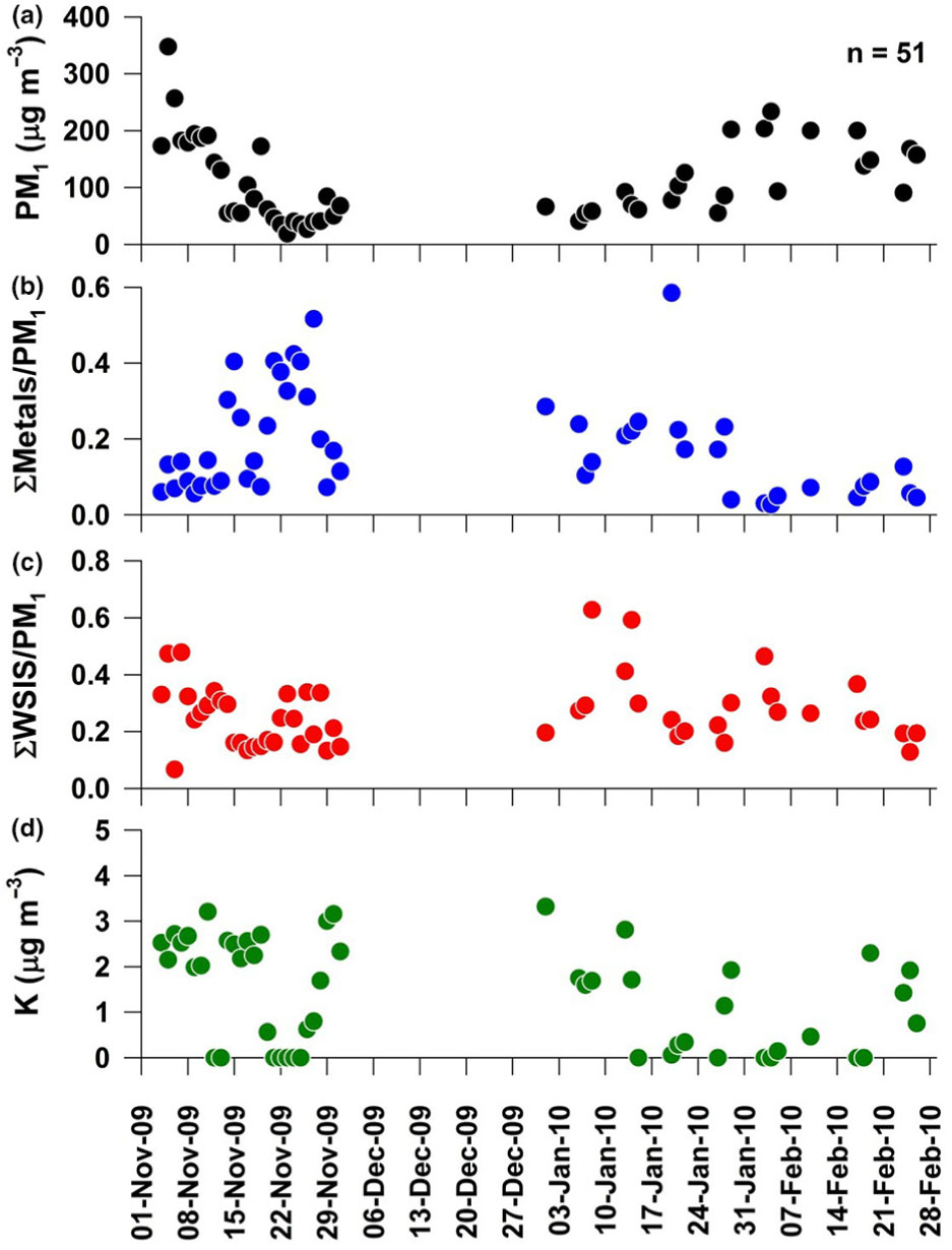
Fig. 1

Aerosol acidity due to non-sea-salt (nss)- is indexed in terms of -to- equivalent ratio less than 1. In general, -to- equivalent ratio of 1 suggests that all is neutralised by . However, -to- equivalent ratio greater than 1 (e.g. most of the data points in this study) suggests that is in excess or is a limiting reactant. In this context, previous studies have suggested that excess can lead to the formation of aerosol phase (Pathak et al., 2009). In this study, -to- equivalent ratio varies from 0.31 to 6.93 (Avg±SD: 2.37±1.57; Fig. 2a) and / mass ratio varies from 0.05 to 1.13 (0.30±0.23; Fig. 2b). It is important to mention here that temporal trends in the variability of / mass ratio follow a quite similar trend to -to- equivalent ratio. This observation is in good agreement with previous studies focusing on secondary aerosol formation (Pathak et al., 2009). Summing up, in this study all is neutralised by at Kanpur location in IGP. Furthermore, temporal variability among , and indicates predominant association of and with (Fig. 2a and b).

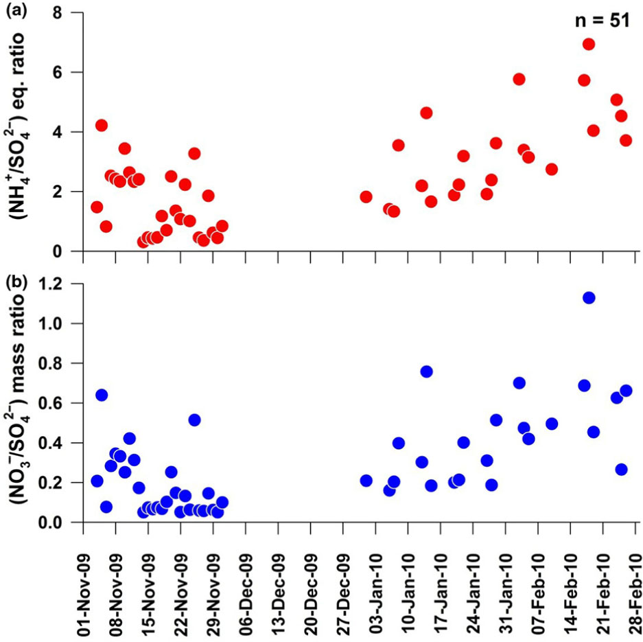
Fig. 2

3.2. Distribution pattern among WSIS: a global perspective

Mass closure of WSIS among , , and Cl⁻ from this study (urban) and some other geographical locations (urban, rural, coastal and high-altitude) in the world is shown in Fig. 3. It is important to mention here that for comparison in PM₁ samples (this study), we have adopted the Aerodyne Aerosol Mass Spectrometer (AMS) data set (wintertime) from European and Chinese locations. As shown in Fig. 3, it is obvious that atmospheric abundance pattern among these WSIS (Avg: 31.40 µg m⁻³) follows a pattern ≈ (40 %) > (14 %) > Cl⁻ (6 %) at the study location (Kanpur; IGP). It can be seen from Fig. 3 that ∑WSIS concentration averages at 8.19 µg m⁻³ at Zurich (urban), 10.04 µg m⁻³ at Payerne (rural) and 2.10 µg m⁻³ at Montsec (a high-altitude location) with a common trend of > ≈ >Cl⁻ (Lanz et al., 2010; Ripoll et al., 2015). Thus, a common feature in IGP at Kanpur and European locations discussed herein is the complete neutralisation of by . In sharp contrast, if we compare the data set from different locations in China, ∑WSIS concentration centres at 44.65, 20.60, 19.69 and 10.33 µg m⁻³ at Beijing (urban), Shenzhen (urban), Kaiping (rural) and HKUST (a coastal location) (He et al., 2011; Huang et al., 2011; Zhang et al., 2014; Li et al., 2015). By and large these data sets from Chinese locations follow a trend > ≈ >Cl⁻. Summing up, owing to the source variability and prevailing meteorological conditions, mass composition of WSIS exhibit a spatial variability. Furthermore, relatively high concentration at Chinese locations has implications on the regional aerosol acidity and organosulphate formation (Surratt et al., 2008).

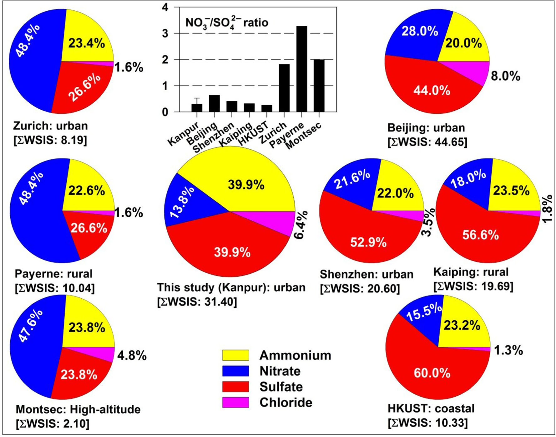
Fig. 3

In this study, at Kanpur location (urban; IGP) / mass ratio averages at 0.30±0.23. This ratio is nearly similar to 0.64 (Beijing; urban), 0.41 (Shenzhen; urban), 0.32 (Kaiping; rural) and 0.26 (HKUST; coastal) in Chinese locations (He et al., 2011; Huang et al., 2011; Zhang et al., 2014; Li et al., 2015). Thus, from this study and those over Chinese locations it is obvious that concentration is more than the concentration during wintertime. In a sharp contrast, / mass ratio of 1.82 (Zurich; urban), 3.27 (Payerne; rural) and 2.00 (Montsec; a high-altitude locations) are reported from different geographical locations during wintertime in Europe (Lanz et al., 2010; Ripoll et al., 2015). These studies suggest dominance of over at those locations in Europe. Thus, excess abundance of (post to neutralisation), volatility of and source variability is attributable to alter / mass ratio on a spatial-temporal scale.

3.3. Source apportionment of PM₁: PMF approach

This study utilises PMF (version 5.0) (Paatero et al., 2014; Rajput et al., 2015) for assessing source apportionment of PM₁ over the study location at Kanpur in IGP. PMF is basically a receptor model and a multivariate factor analysis tool which only considers non-negative data matrix. The model works on assumption of mass conservation, and therefore, utilises a mass balance approach which leads to identify and quantify the plausible sources of atmospheric aerosols. The fundamental logic of PMF is based on the estimation of point-by-point least square minimisation which facilitates to extract the information from each and every species and sample. PMF analysis splits each data matrix into two matrices: one is the source contribution matrix (G) and the other one is source profile matrix (F). Mathematically,

where i can vary from 1, 2 … n samples; j from 1, 2 … m species and k from 1, 2 … p factors. E is the residual matrix.

There are two modes of analysis in PMF: true and robust mode. In true mode, PMF analysis is carried out with equal weight on all data points whereas in the robust mode outliers are given less weight. Minimisation of Q value has been achieved (Supplementary Fig. 1a) in this study (robust mode) using the following approach:

where, h _ij (robustness) is introduced to reduce the effect of outliers.

To estimate uncertainties we have adopted the following approach:

where p _j is uncertainty proportional parameter and MDL _j is method detection limit for the jth species (Gupta and Mandaria, 2013).

One of the important aspects of PMF involves the Fpeak analysis. Actually, there may exist a non-singular matrix T (of dimension p×p) such that when T and T⁻¹ are multiplied to make solution matrices G and F, respectively, the resulting matrices G* and F* which also satisfies the non-negative constrain, and thus, will form an alternate solution. Fpeak analysis is assessed to remove rotational ambiguity in the model output. At present, we have used Fpeak from +1 to −1 (Supplementary Fig. 1b).

PMF was run (with 15 % uncertainty) for present data set (n=51) with 21 parameters as input to the model. Two species (As, Co) were marked as ‘Bad’ because of too many missing values. S/N ratio for the remaining species was observed and species for which S/N ratio was greater than 2.0 has been marked as ‘Strong’ (Fig. 4a). PMF analysis has been carried out with 20 run and six factor solutions. With this methodology, it was observed that all base number runs were converging and also all Q run values were between 10 % range of minimum Q value (Fig. 4b). This is an indication of a stable Q robust value. Thus, 20 run number and six factor solution fits model with a good measure.

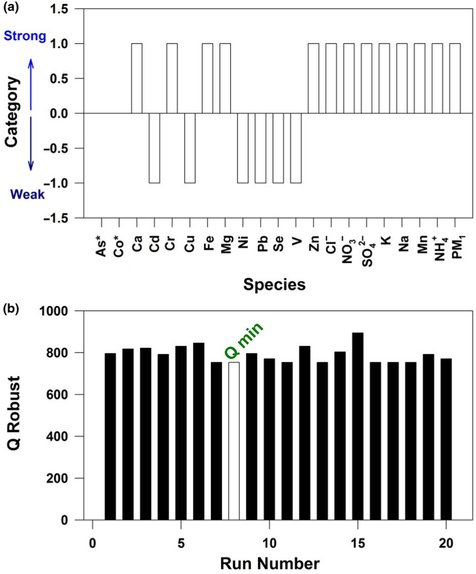
Fig. 4

Furthermore, in the base model result, residual analysis was inspected. For a good model fit, the residual should follow a normal distribution pattern. It was observed that Pb, Se, V, Cd and Ni are exceeding +3 to −3 range of residual analysis, and therefore, these species are marked as ‘Weak’ and the model was re-run under identical conditions. This time it was observed that all species are in the range of +3 to −3. Moreover, regression analysis for different species was also carried out to assess R ² values. It was observed that only Cu has a low R ² value (<0.1). Therefore, this species is marked as ‘Weak’ species (Fig. 4a) and the model was re-run under an identical condition to achieve global minima Q value.

Summing up, PMF analysis has been carried out with a model uncertainty of 15 % to achieve global minima for Q (Robust; Fig. 4b). Finally, it has been assured that all runs are converging and all Q robust values fall in the range of 10 % of minimum Q robust value. Most of the species were found in the range of +3 to −3 in residual analysis (16 out of 21). Thus, residual analysis shows that our results (PMF) represent a good fit based on the normal distribution pattern for most of the species (between +3 and −3). A normal distribution pattern in residual analysis indicates for non-randomness of data. R ² value between observed and predicted PM₁ mass concentration was observed as 0.76, suggesting that PMF analysis is a good fit model in this study (n=51).

3.4. Overall source contribution of PM₁

Based on PMF analysis, in this study, we show (Fig. 5a–f) percentage contribution of all resolved sources (n=6) influencing aerosol contribution at Kanpur site during winter. The temporal variability of each source contribution (Fig. 5) facilitates to better understand predominant impacts of a particular source on a given sampling event. We will now discuss the factor loading of essential constituents and overall source contribution of PM₁. Subsequently, we will discuss source apportionment in conjunction with AMBT.

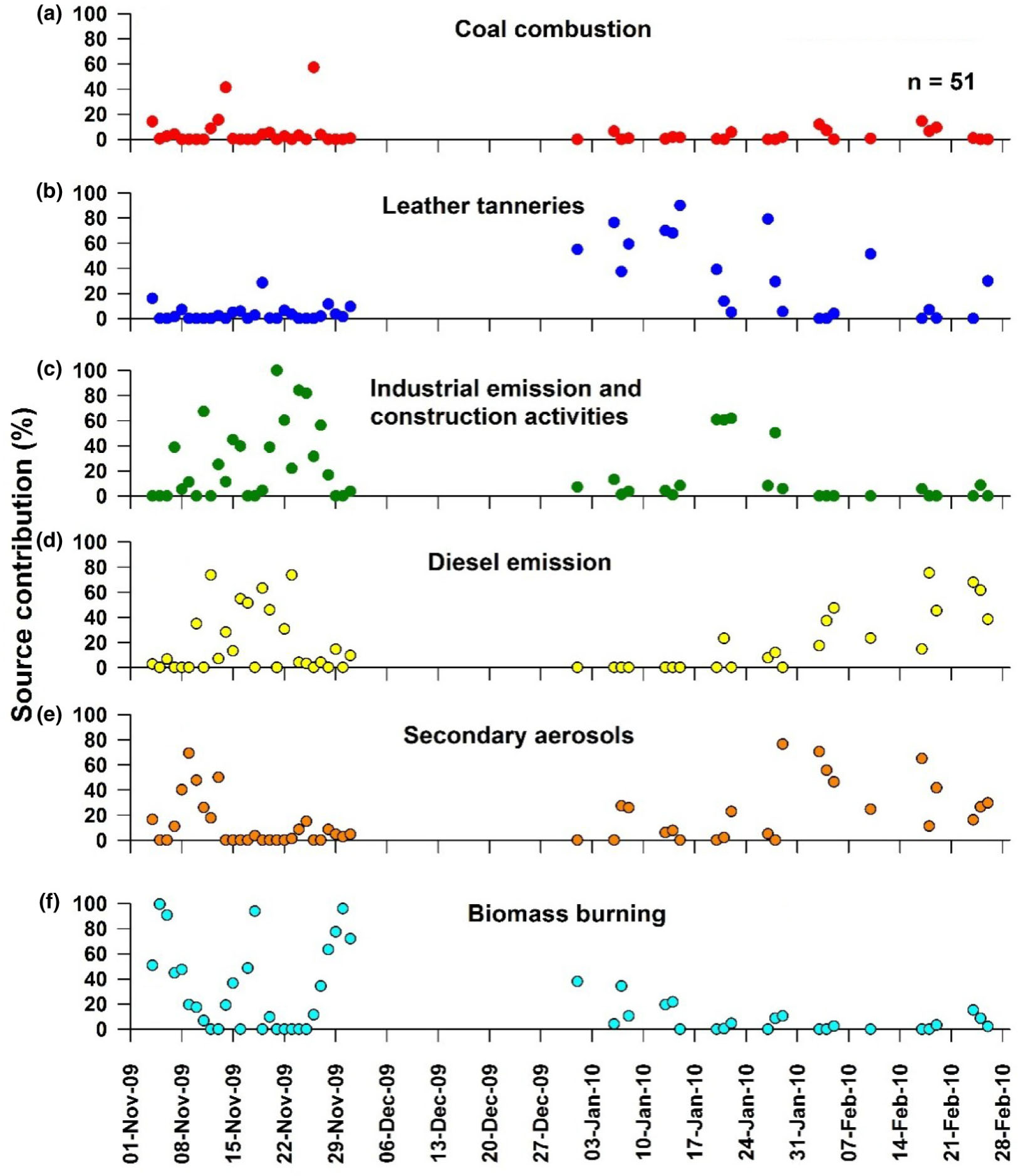
Fig. 5

3.5. Percentage source contribution in conjunction with AMBT

HYSPLIT (Hybrid Single Particle Lagrangian Integrated Trajectory) model is run to infer about the AMBT at receptor site (Draxler and Rolph, 2003). 5d AMBTs (1000 m) above mean sea level, or amsl) are shown in Fig. 6 for all sampling days in this study. From Fig. 6, it is obvious that NW-winds favor predominantly long-range transport of air pollutants from upwind IGP during November–February. During the same period, previous studies have assessed the impact of long-range transport across IGP in marine atmospheric boundary layer over the BoB. It is important to mention that these AMBTs show pathways quite similar to those inferred from MODIS satellite imageries depicting advection of haze over the BoB (Ramanathan et al., 2007).

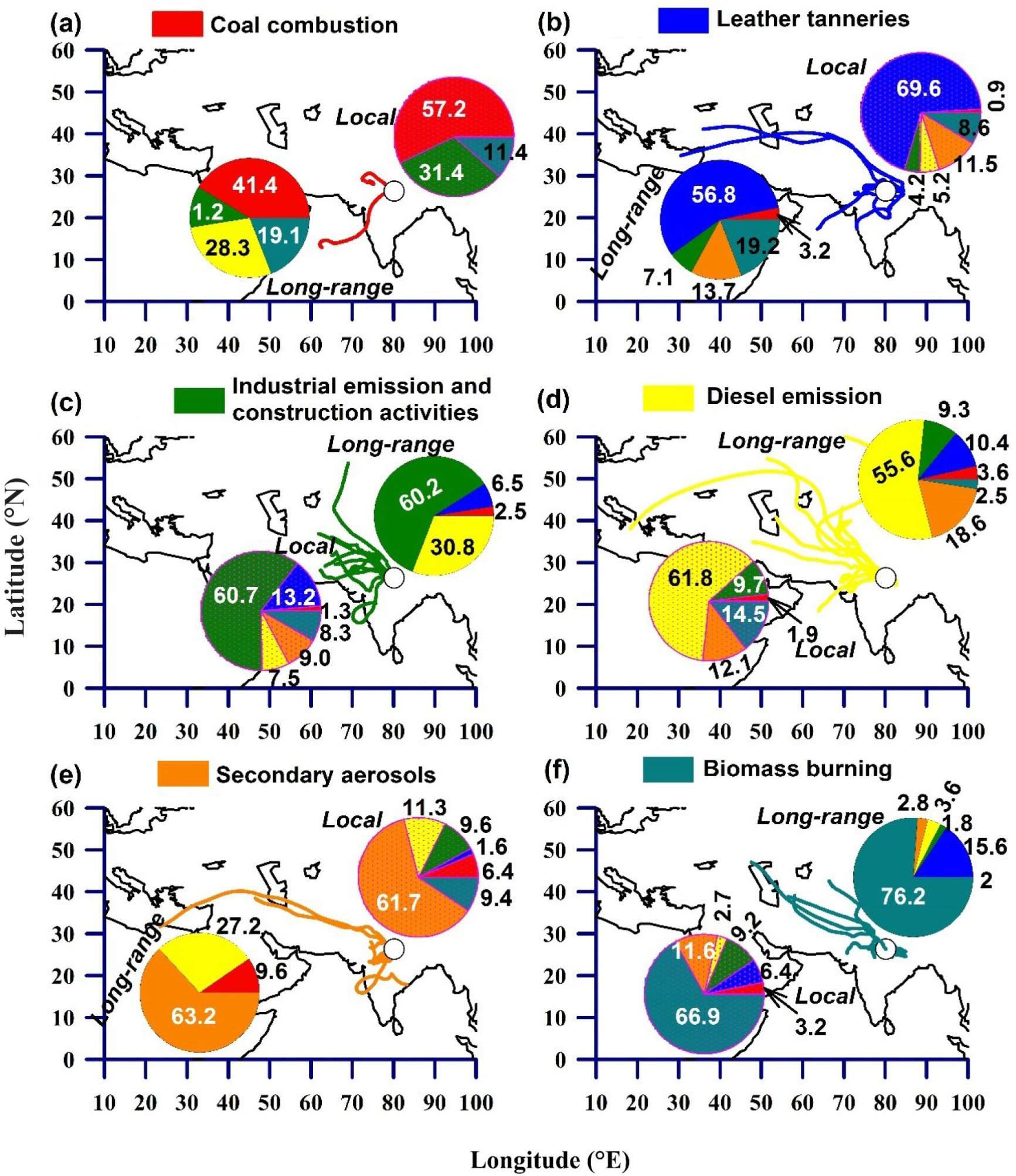
Fig. 6

As aforementioned that for n=51 sampling events at Kanpur, PMF analysis shows aerosols contribution fromsix sources (Fig. 5). As shown in Fig. 5, on each given sampling day a particular source contributes predominantly. So, we have sorted out n=51 sampling events based on the prominent source on that day and coupled this information with AMBT (Fig. 6). Thus, for each source (Fig. 5), we couple information on AMBT to characterise the source contribution (%) into local sources (short AMBT) and long-range transport (long AMBT; Fig. 6). For example, there is a difference in source contribution associated with local versus long-range transport (through west-coast of India) event when coal combustion is the predominant source (local: 57 %; long-range transport: 41 %) of PM₁ at Kanpur (Fig. 6a). Likewise, events with pronounced impact from leather tanneries show distinct source contribution for local (70 %) versus air-mass originated from the Middle East (57 %; Fig. 6b). Events with predominance from industrial emission and construction activities (60 %; Fig. 6c), diesel emission (local: 62 %; long-range transport: 56 %; Fig. 6d) and secondary aerosols (60 %; Fig. 6e) also show differences associated with short and long AMBTs (originating from Middle East, Kazakhstan and Russia). It is important to mention here that for most of the above cases during the study period (November–February), long-range transport was associated with NW-winds. Interestingly, biomass burning emission contribution varies from ~10 to 20 %, while the other sources are predominant and the origin of air-masses point to source region other than the upwind IGP. However, there are events when the impact from biomass burning emissions is predominant (local: 67 %; long-range transport: 76 %; Fig. 6f). Interestingly, not only the events associated with long-range transport from upwind IGP but the local sources also relate to the predominance of biomass burning emissions on some sampling events (Fig. 6f). Thus, our study shows that there are local sources of biomass burning emissions too in and around the Kanpur. Summing up, this study assesses aerosol chemical characteristics and impact of sources coupled with AMBTs in central IGP (Kanpur).