
1. Introduction
During the past century, increased human activities have caused large changes in the global climate system, such as an increase in mean air temperature, a decrease in diurnal temperature range, a redistribution of precipitation and intensification of extreme climate events (IPCC, 2013). Terrestrial ecosystems can not only respond to the climate change, but they also regulate the changing rate of the climate because they absorb 30 % of the anthropogenic CO2 emissions and determine the interannual fluctuation in the atmospheric CO2 concentration growth rate (Canadell et al., 2007; Le Quéré et al., 2014; Ahlström et al., 2015). The interannual variability (IAV) in the net ecosystem exchange of CO2 (NEE) is widely observed in eddy-flux networks, and its drivers have been attributed to a series of climatic and biotic factors (Barr et al., 2007; Pintér et al., 2008; Richardson et al., 2009; Yuan et al., 2009; Dragoni et al., 2011; Humphreys and Lafleur, 2011; Wu et al., 2013). However, model simulations of the IAV in NEE is one of the most urgent and challenging scientific tasks because of the lack of substantial understanding of the intrinsic predictability of IAV in the terrestrial ecosystem carbon (C) cycle (Luo et al., 2015).
The difficulty in predicting the IAV in NEE might result partially from the failure of models to represent the temporal evolution of ecophysiological (e.g. physiological and phenological) factors, which outweigh the climatic factors in most eddy-flux sites at the interannual scale (Shao et al., 2015). Although empirical and semi-empirical research suggests that the ecophysiological properties of ecosystems should be taken into consideration for better simulation of the IAV in C fluxes (Kuzyakov and Gavrichkova, 2010; Migliavacca et al., 2011; Xia et al., 2015), the results from modelling studies indicate that it is still troublesome to predict the temporal changes in the biotic factors or ecophysiological properties of ecosystems (Richardson et al., 2012). Therefore, appropriately representing the dynamics of ecosystem ecophysiology embraces the opportunity to address the issues raised by the IAV in NEE.
The ecophysiological factors that are directly related to the IAV in NEE include photosynthetic and respiratory parameters (hereafter referred as the physiological parameters) that characterize the responses of photosynthesis and respiration to the climatic variations (Shao et al., 2015). Other biotic factors (e.g. biotic disturbance) can only affect the IAV in NEE by changing these parameters. The changes in the physiological parameters can be induced by climatic variations, internal changes in the ecosystem and natural or human disturbances (Richardson et al., 2007; Shao et al., 2015). Among these, the effects of climatic factors on physiological parameters reflect the ecophysiological regulation of ecosystem C cycling by the climatic variations, which occur from the leaf to the ecosystem level (Niu et al., 2012; Wythers et al., 2013; Way and Yamori, 2014; Yamori et al., 2014). At the ecosystem level, a handful of studies have shown that the seasonality of physiological parameters, such as the maximum carboxylation rate (V cmax, maximum velocity of the carboxylase), maximum photosynthetic rate (A m , light-saturated photosynthetic rate at the ambient CO2 concentration), light use efficiency, water use efficiency (WUE), reference respiratory rate at 10 °C (R 10) and temperature sensitivity (Q 10) were related to radiation, temperature and water conditions in some ecosystems (Aber et al., 1996; Barr et al., 2007; Ricciuto et al., 2008; Yu et al., 2008; Ju et al., 2010; Shao et al., 2014; Shi et al., 2014; Peichl et al., 2015). At a larger temporal scale (interannual), the optimum temperature of NEE, the Michaelis constant of gross primary productivity (GPP), WUE and R 10 have also been related to the climatic variations (Bahn et al., 2008; Niu et al., 2011, 2012; Shao et al., 2014).
The effects of climate on the IAV in C fluxes mediated by physiological parameters can be considered to be the indirect climatic effects, the strength of which depends on both the correlations between climatic variables and physiological parameters, and the correlations between physiological parameters and C fluxes. If the indirect climatic effects are important contributors to the IAV in C fluxes, the performance of a model can be improved by expressing the physiological parameters as functions of the climatic variables (Ricciuto et al., 2008; Shao et al., 2014). Whether this approach will work or not largely depends on the explicit paths through which the climate directly and indirectly impacts the C fluxes. However, these paths have not been synthetically investigated within eddy-flux networks. To address this issue, we applied a path analysis to 481 site-years of flux data from 65 sites in order to examine the direct and indirect effects of climatic variations on the IAV in NEE and its components (GPP and ecosystem respiration (RE)). Path analysis is a statistical method that is able to quantify the direct and indirect dependencies between or among many variables under consideration (i.e. climatic variables, physiological parameters and C fluxes in this study). The main questions we focused on were: (1) how and to what extent does the climate directly and indirectly affect IAV in C fluxes; and (2) how are these relationships affected by ecosystem characteristics, such as biome types and multi-year water conditions?
2. Materials and methods
2.1. Data sources
The original half-hourly C flux and auxiliary climate data were obtained from AmeriFlux (www.ameriflux.lbl.gov/), CarboEurope (www.europe-fluxdata.eu) and ChinaFLUX (www.chinaflux.org). Only the sites with data for ≥5 yr were selected. In total, there were 481 site-years of data belonging to 65 eddy covariance measurement sites from 1992 to 2010 (Table 1, Supplementary Fig. 1). These sites covered a large range of geographical positions and climatic conditions, which can be broadly classified into evergreen needleleaf forests, deciduous broadleaf forests, evergreen broadleaf forests, mixed forests, shrublands, grasslands and croplands (Table 1). The original data included CO2 flux (Fc), friction velocity, photosynthetically active radiation (PAR) or global radiation, air temperature (Ta), soil temperature (Ts), annual precipitation (PPT), relative humidity (RH), vapour pressure deficit (VPD) and latent heat flux (LE).
Table 1. Information of study sites
US-Blo38.90−120.631315ENF911.91073Goldstein et al. (2000)US-Dk335.98−79.09163ENF815.01050Stoy et al. (2008)US-Fmf35.14−111.732160ENF59.7521Dore et al. (2008)US-Fuf35.09−111.762180ENF58.9497Dore et al. (2008)US-Ho145.20−68.7460ENF136.7840Richardson et al. (2009)US-Ho245.21−68.7591ENF116.6842Xiao et al. (2005)US-Ho345.21−68.7361ENF56.5877Davidson et al. (2006)US-Me244.45−121.561253ENF97.4441Thomas et al. (2009)US-NC235.80−76.6712ENF515.81212Noormets et al. (2010)US-NR140.03−105.553050ENF102.4663Blanken et al. (2009)US-SP329.75−82.1636ENF1120.11034Powell et al. (2008)DE-Tha50.9613.57380ENF127.6820Prescher et al. (2010)DE-Wet50.4511.46703ENF76.6967Rebmann et al. (2010)ES-ES139.35−0.321ENF517.5495Reichstein et al. (2005)FI-Hyy61.8524.29185ENF114.8702Suni et al. (2003)FI-Sod67.3626.64189ENF71.1425Aurela (2005)FR-Pue43.743.60211ENF813.6904Allard et al. (2008)IT-Cpz41.7112.389ENF815.0729Garbulsky et al. (2008)NL-Loo52.175.7425ENF1010.3843Dolman et al. (2002)RU-Fyo56.4632.92265ENF95.2762Milyukova et al. (2002)SE-Nor60.0917.4828ENF56.4486Lagergren et al. (2005)CN-Qia26.74115.06100ENF718.31139Zhang et al. (2011)US-Bar44.06−71.29272DBF57.41330Jenkins et al. (2007)US-Dk235.97−79.10168DBF715.21097Stoy et al. (2008)US-Ha142.54−72.17340DBF158.51153Urbanski et al. (2007)US-MMS39.32−86.41275DBF512.71186Dragoni et al. (2011)US-MOz38.74−92.20219.4DBF513.01035Yang et al. (2010)US-Slt39.91−74.6030DBF512.41032Hollinger et al. (2010)US-Syv46.24−89.35540DBF54.5696Desai et al. (2005)US-UMB45.56−84.71234DBF67.2412Hardiman et al. (2011)US-WCr45.91−90.08515DBF75.7744Cook et al. (2004)DE-Hai51.0810.45433DBF88.3803Kutsch et al. (2008)FR-Hes48.677.07293DBF1210.4918Granier et al. (2000)IT-Ro142.4111.93153DBF715.5769Rey et al. (2002)CN-Din23.17112.53240EBF620.11481Zhang et al. (2010)BE-Bra51.314.5215MF911.4792Carrara et al. (2003)BE-Vie50.316.00491MF118.3719Aubinet et al. (2001)CH-Lae47.488.37645MF58.3605Eugster et al. (2007)DK-Sor55.4911.6435MF138.7656Pilegaard et al. (2001)CN-Cha42.40128.10738MF63.9498Guan et al. (2006)US-Los46.08−89.98480SHR63.7716Sulman et al. (2009)MX-Lpa24.13−110.4421SHR523.4137Bell et al. (2012)US-Aud31.59−110.511469GRA615.9366Krishnan et al. (2012)US-Bkg44.35−96.84510GRA56.3540Gilmanov et al. (2005)US-Dk135.97−79.09168GRA715.11022Stoy et al. (2008)US-FPe48.31−105.10634GRA85.7391Gilmanov et al. (2005)US-Fwf35.45−111.772270GRA58.4562Dore et al. (2008)US-SRM31.82−110.871116GRA719.0324Scott et al. (2009)US-Ton38.43−120.97177GRA916.9504Ma et al. (2007)US-Var38.41−120.95129GRA915.9493Xu and Baldocchi (2004)US-Wkg31.74−109.941531GRA617.2274Scott et al. (2010)AT-Neu47.1211.321095GRA76.9731Wohlfahrt et al. (2008)DE-Gri50.9513.51385GRA57.8901Prescher et al. (2010)DK-Lva55.6812.0815GRA59.0655Gilmanov et al. (2007)HU-Bug46.6919.60106GRA610.3499Nagy et al. (2007)NL-Ca151.974.931GRA611.0759Gilmanov et al. (2007)CN-Dan29.6791.334333GRA52.47470Xu et al. (2007)CN-Hab37.62101.283220GRA6−0.8484Kato et al. (2006)US-ARM36.61−97.49314CRO715.3658Fischer et al. (2007)US-Bo140.01−88.29219CRO1111.6748Hollinger et al. (2005)US-Ne141.17−96.48361CRO810.7846Suyker et al. (2004)US-Ne241.16−96.47362CRO810.2872Suyker et al. (2004)BE-Lon50.554.74165CRO511.2611Moureaux et al. (2006)DE-Geb51.1010.91157CRO69.9503Anthoni et al. (2004)DE-Kli50.8913.52478CRO67.7951Prescher et al. (2010)
[i] Lat, latitude; Long, longitude; Alt, altitude; Eco, ecosystem type; n, data record length; Ta, mean annual air temperature; PPT, annual precipitation; ENF, evergreen needleleaf forest; DBF, deciduous broadleaf forest; EBF, evergreen broadleaf forest; MF, mixed forest; SHR, shrubland; GRA, grassland; CRO, cropland.
2.2. Data processing
To obtain the annual values for the C fluxes, climatic variables and physiological parameters, several data processing procedures were applied. The original half-hourly Fc data were first spike-screened by using the median of absolute deviation as a spike estimator based on the double differenced time series (Papale et al., 2006). Next, the night-time Fc was rejected if the friction velocity was lower than a threshold, which was determined by a 99 % threshold criterion method based on each year's night-time data (Reichstein et al., 2005; Papale et al., 2006). After that, the artificial neural network model with a feed-forward back-propagation algorithm and sigmoid transfer function was applied to partition the NEE into GPP and RE, and to fill the gaps (Shao et al., 2015). The artificial neural network model was trained and validated separately for each year's daytime and night-time data. The input variables of the night-time model were Ts, RH and four seasonal indices, which represented the four seasons (Papale and Valentini, 2003), and the output variable was the night-time RE. The hidden layer had six nodes. The dataset was randomly divided into a training dataset (70 %) and a validation dataset (30 %). This process was repeated 20 times, and the median of 20 simulated outputs was used to fill the gaps in night-time RE and to simulate the daytime RE. The input variables of the daytime model were PAR, Ta, RH and the four seasonal indices, and the output variable was GPP (daytime RE – NEE). Six nodes were set in the hidden layer. The training and validation procedures were repeated 20 times and the median of the simulated GPP was used to fill the GPP gaps. The NEE gaps were filled by the gap-filled RE – GPP. Finally, the gap-filled NEE, GPP and RE, as well as the corresponding climatic variables, were integrated or averaged on an annual basis.
The physiological (photosynthetic and respiratory) parameters used in this study were the maximum photosynthetic rate (A m ), apparent quantum yield (α), WUE, R 10 and Q 10. A m , α, R 10 and Q 10 were derived from the Michaelis–Menten and Q 10 equations (Falge et al., 2001; Richardson and Hollinger, 2005):
These equations were parameterised on the basis of 30-d moving windows with a step of 1 d, and only the GPP and RE partitioned from the NEE data were used. The estimated parameters with coefficients of variation larger than 0.5 were excluded (Reichstein et al., 2005) and the median of a certain parameter in a year was considered to be the annual value of the parameter. The WUE is the ratio of GPP to evapotranspiration (ET, calculated from LE [ET (mm/day)=LE (W/m2)/28.94]) (Yuan et al., 2009).
2.3. Path analysis
The dataset used in this study had previously been analysed by Shao et al. (2015) but with different methods and aims. The additive model in Shao et al. (2015) aimed to quantify the relative contribution of climatic and biotic factors to IAV in C fluxes, but it could not identify the paths through which the climate directly and indirectly affected the C fluxes. Therefore, in order to elucidate the direct and indirect effects of climatic variables on the IAV in C fluxes, we applied path analysis, which is an extension of regression model and can deal with multiple casual relationships between or among correlated variables (Shipley, 2004), to the dataset in Shao et al. (2015). Theoretically, path analysis can incorporate nonlinear interactions between climatic variables and C fluxes by using nonlinear functional forms. However, in our study, no nonlinear relationships between variables were found at the interannual scale, though they might exist at shorter temporal scales. The standardised path coefficient (ρ, the path coefficient when all the variables were standardised before the analysis), which is an analogy of the correlation coefficient, was used to quantify the effect size of one variable on another.
Shao et al. (2015) suggested that the correlations between climatic and biotic factors might depend on biome types and multi-year water conditions. Therefore, the study sites were grouped into evergreen needleleaf forests, deciduous broadleaf forests, grasslands and croplands according to their plant function type. In addition, we used the water balance index (WBI), which is the difference between evapotranspiration and precipitation (Law et al., 2002), to group the sites into wet (WBI below −500 mm), moist (−500 mm<WBI<0 mm) and dry (WBI>0 mm) ecosystems according to their multi-year water conditions. In order to exclude the influence of different magnitudes of the variables among ecosystems, the annual climatic variables, physiological parameters and C fluxes in each site were first standardised by subtracting the mean and then dividing it by the standard deviation of the multi-year data. Path analysis was then applied to each group separately.
For each ecosystem group, two path models were conducted: one for NEE and another for GPP and RE. The use of two models instead of one is because even though some variables are critical to GPP and RE, they may not necessarily be important to NEE. The potential paths in the models mainly included three aspects: the direct effects of climatic variables on C fluxes, the direct effects of climatic variables on physiological parameters and the direct effects of physiological parameters on C fluxes. The first of these three groups were the direct climatic effects; the latter two together characterised the indirect climatic effects on the IAV in C fluxes. In addition, we also considered the regulation of GPP on RE (Supplementary Tables 1 and 2).
The potential paths were based on the following considerations (Supplementary Tables 1 and 2). (1) For the causal paths from climate to C fluxes, five climatic variables (PAR, Ta, Ts, VPD and WBI) were considered to affect NEE and GPP directly, whereas Ta, Ts, VPD and WBI affect RE (precipitation was not considered as an explanatory variable because its effects were actually mediated by water availability, which was the opposite of WBI). (2) The IAV in photosynthetic parameters (A m , α and WUE) may be induced by changes in radiation (PAR), temperature (Ta, Ts) and water conditions (VPD, WBI), whereas the IAV in respiratory parameters (R 10 and Q 10) might be driven by temperature and water conditions. (3) The photosynthetic and respiratory parameters may influence GPP and RE, respectively, and both kinds of physiological parameter may be important to NEE. (4) The correlation between GPP and RE was found within and across ecosystems (Chen et al., 2015), and may be caused by the substrate supply of photosynthesis to both autotrophic and heterotrophic respiration (Schimel et al., 1994). Therefore, we also assumed that GPP might influence R 10. However, autotrophic and heterotrophic respiration might be driven by different factors and correlated differently with GPP, which might result in relationships other than that between GPP and R 10. Thus, the control of GPP on RE was also included in the path model. (5) Water availability in autumn and winter might influence the plants’ phenology in the next spring and thus was important to the C fluxes in the next year (Gordo and Sanz, 2005). Therefore, the lag effects of autumn–winter WBI on next year's C fluxes and physiological parameters were considered.
The full path models contained too many paths compared to the sample size, which might have caused an overparameterisation problem or may have even failed to derive any statistical tests. Therefore, we simplified the model structure by excluding the paths where the corresponding bivariate correlation coefficients (r) were larger than −0.1 and smaller than 0.1. A path model with the remaining paths was conducted, and the standardised path coefficients (ρ) and the corresponding p-values were calculated via maximum likelihood estimation (Beaujean, 2014). To obtain the most parsimonious path model for each ecosystem group, the non-significant paths were excluded recursively by dropping the path with the largest non-significant p-value each time and then re-parameterising the new model. This procedure was repeated until all the paths were significant (p<0.05). In order to make the results among ecosystem groups comparable, we constructed final path models that contained all the significant paths in the most parsimonious models of all the ecosystem groups to be compared. This treatment helped to eliminate the uncertainty caused by variable selection. The path analysis was achieved by using the package lavaan in R software (Rosseel, 2012; R Core Team, 2014).
3. Results
3.1. Direct and indirect climatic effects in different biomes
In all the biomes being studied (evergreen needleleaf forests, deciduous broadleaf forests, grasslands and croplands), the maximum photosynthetic rate (A m ) was the most important factor for the IAV in C fluxes (the standardised path coefficient (ρ) as an analogy of the correlation coefficient fell between −0.32 and −0.68 for NEE and 0.72–0.85 for GPP), which was mainly induced by the variation in VPD (Figs. 1 and 2). For the IAV in RE, the most important drivers were GPP (ρ=0.47–0.67) and reference respiratory rate (R 10, ρ=0.24–0.29 except for croplands; Fig. 2). Though we also considered the lag effects of autumn–winter WBI on the physiological parameters and C fluxes in the next year (Supplementary Table 3), they were not selected in the final path models.
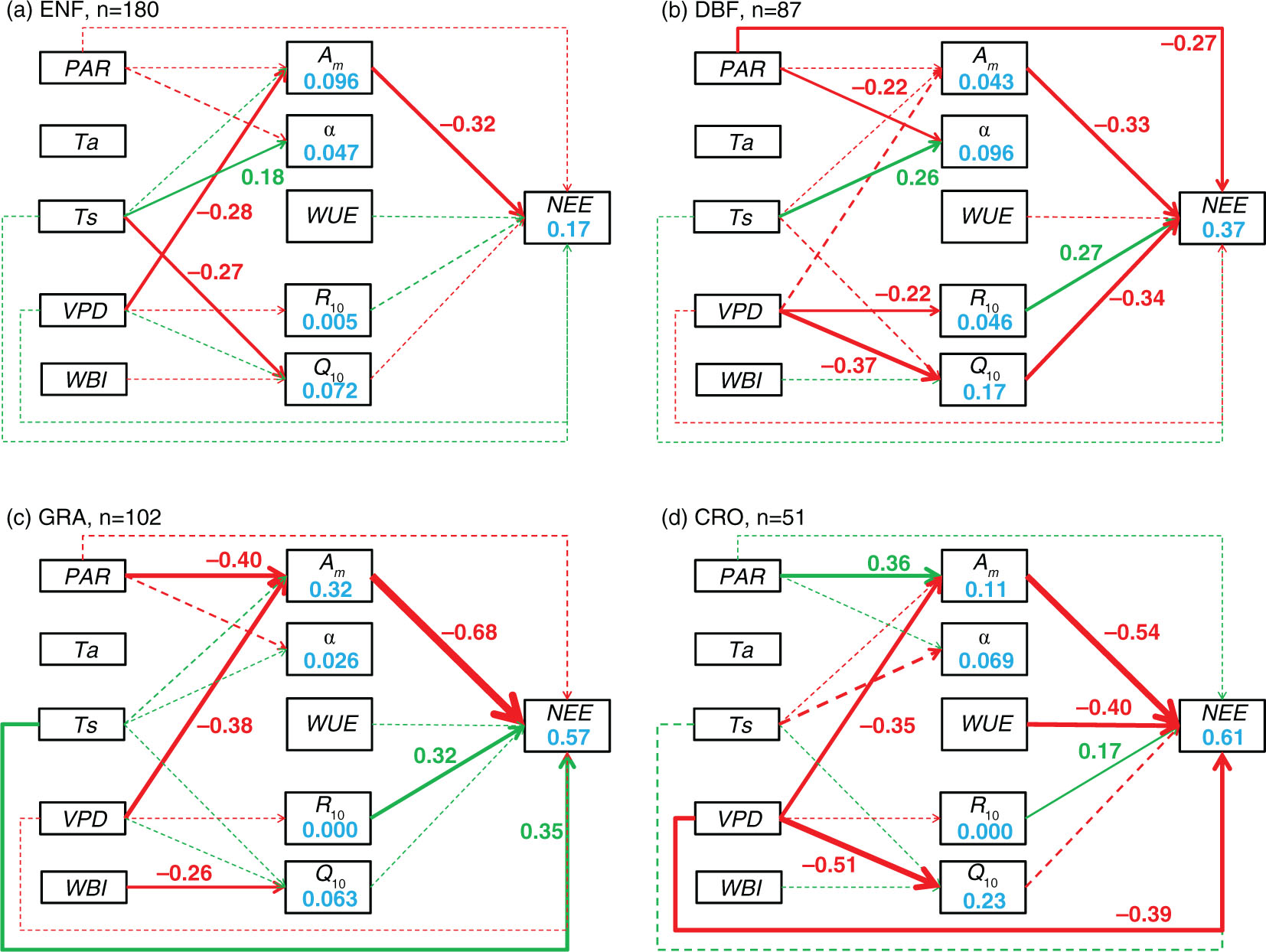
Fig. 1
The direct and indirect effects of climatic variation on the interannual variability (IAV) in net ecosystem exchange (NEE) for evergreen needleleaf forests (a), deciduous broadleaf forests (b), grasslands (c) and croplands (d). Green and red lines represent positive and negative effects, respectively. Solid and dashed lines represent significant (p<0.05) and non-significant (p≥0.05) effects, respectively. The values beside the paths are the standardised (0–1) path coefficients (ρ), which are only shown for significant effects. PAR, photosynthetically active radiation; Ta, air temperature; Ts, soil temperature; VPD, vapour pressure deficit; WBI, water balance index; A m, maximum photosynthetic rate; α, apparent quantum yield; WUE, water use efficiency; R 10, reference respiratory rate at 10 °C; Q 10, temperature sensitivity.
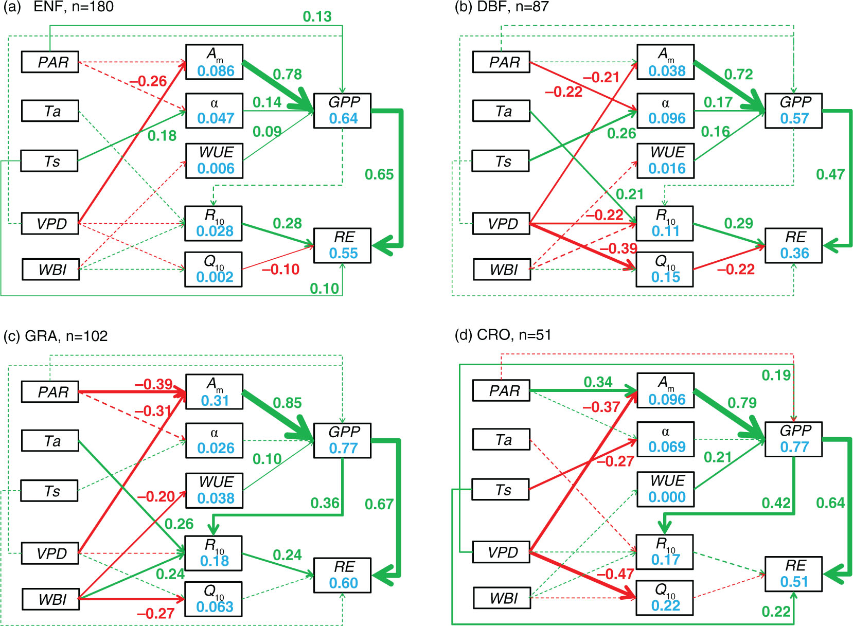
Fig. 2
The direct and indirect effects of climatic variation on in the interannual variability (IAV) in gross primary productivity (GPP) and ecosystem respiration (RE) for evergreen needleleaf forests (a), deciduous broadleaf forests (b), grasslands (c) and croplands (d). Green and red lines represent positive and negative effects, respectively. Solid and dashed lines represent significant (p<0.05) and non-significant (p≥0.05) effects, respectively. The values beside the paths are the standardised (0–1) path coefficients (ρ), which are only shown for significant effects. PAR, photosynthetically active radiation; Ta, air temperature; Ts, soil temperature; VPD, vapour pressure deficit; WBI, water balance index; A m, maximum photosynthetic rate; α, apparent quantum yield; WUE, water use efficiency; R 10, reference respiratory rate at 10 °C; Q 10, temperature sensitivity.
There were also different direct and indirect paths from climate to C fluxes among biomes. For example, a positive correlation between temperature and apparent quantum yield (α), as well as a negative correlation between temperature sensitivity (Q 10) and RE, was only found in forests, while the controls of GPP on reference respiratory rate (R 10) only appeared in non-forests (Fig. 2). Compared with deciduous broadleaf forests, the evergreen needleleaf forests showed direct climatic effects on C fluxes (PAR on GPP, and Ts on RE), while there were more significant indirect climatic effects in deciduous broadleaf forests than in evergreen needleleaf forests (Fig. 2a and b). Although PAR influenced the maximum photosynthetic rate in both grasslands (ρ=−0.39) and croplands (ρ=0.34) within non-forests, it did so in opposite directions. In addition, the indirect climatic effects on RE in grasslands were not found in croplands (Fig. 2c and d).
3.2. Direct and indirect climatic effects in ecosystems with different aridity
The direct and indirect effects of climate on IAV in C fluxes were also different among ecosystems with different multi-year water conditions (Fig. 3). Overall, the moist ecosystems had more complicated direct and indirect paths than wet and dry ecosystems. Compared with wet ecosystems, the IAV in GPP of moist and dry ecosystems can be induced by apparent quantum yield (α, an indicator of light use efficiency, ρ=0.08 and 0.17, respectively) and WUE (ρ=0.13 and 0.24, respectively), and the IAV in RE can be induced by reference respiratory rate (R 10, ρ=0.31 and 0.25, respectively). On the other hand, direct effects of WBI on RE were found in moist (ρ=−0.10) and dry (ρ=−0.18), but not wet ecosystems.
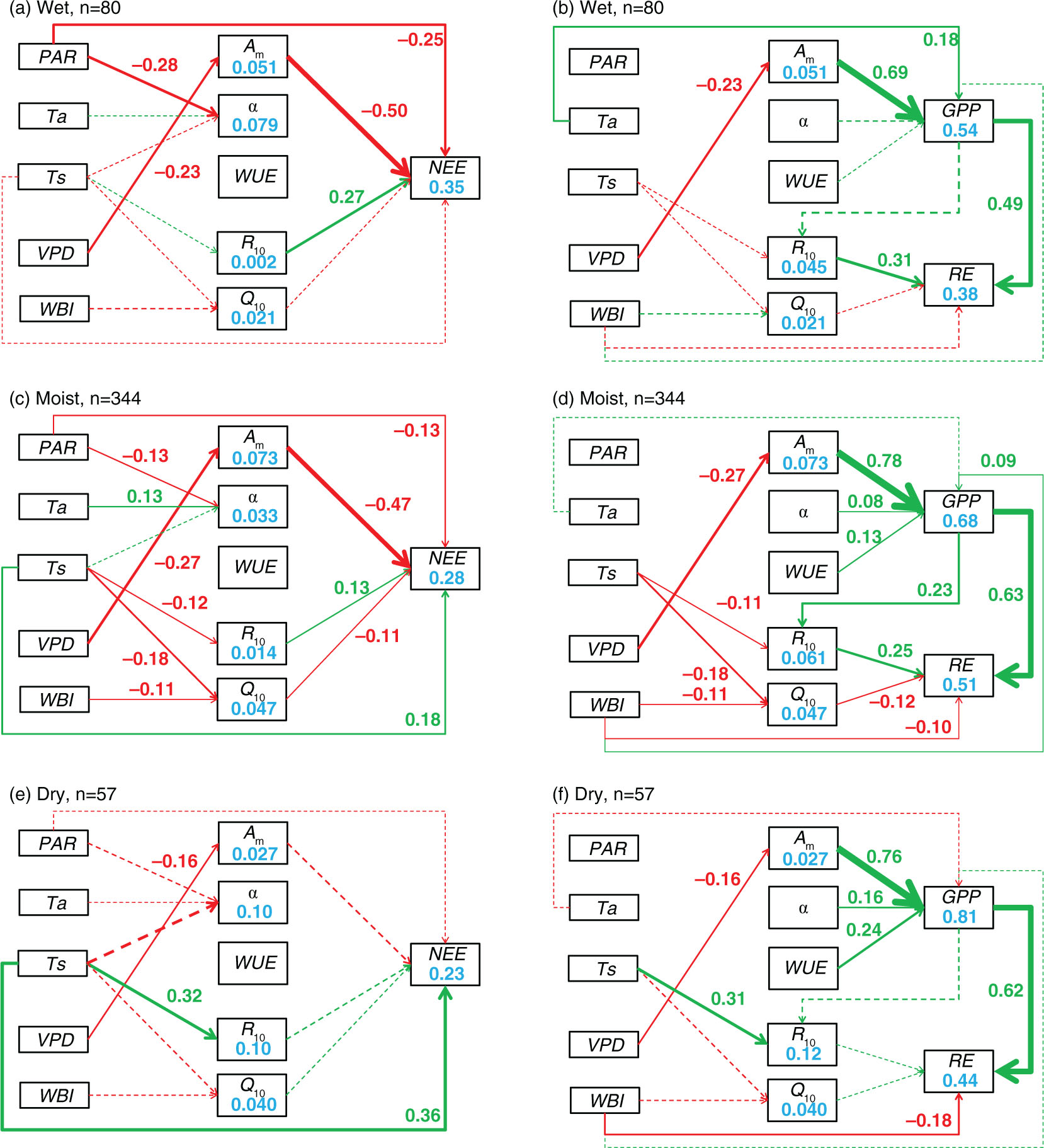
Fig. 3
The direct and indirect effects of climatic variation on the interannual variability (IAV) in net ecosystem exchange (NEE, a–c), gross primary productivity (GPP) and ecosystem respiration (RE, d–f) for wet (water balance index, or WBI, below −500 mm; a, d), moist (−500 mm<WBI<0 mm; b, e), and dry (WBI>0 mm; c, f) ecosystems. Note that a larger WBI indicates a drier environment. Green and red lines represent positive and negative effects, respectively. Solid and dashed lines represent significant (p<0.05) and non-significant (p≥0.05) effects, respectively. The values beside the paths are the standardised (0–1) path coefficients (ρ), which are only shown for significant effects. PAR, photosynthetically active radiation; Ta, air temperature; Ts, soil temperature; VPD, vapour pressure deficit; WBI, water balance index; A m, maximum photosynthetic rate; α, apparent quantum yield; WUE, water use efficiency; R 10, reference respiratory rate at 10 °C; Q 10, temperature sensitivity.
3.3. Model performance
The results derived from the NEE model were generally consistent with those from the GPP and RE model, but with some discrepancies (Figs. (1–3)). For example, the complicated indirect climatic effects in grasslands seen in the GPP and RE model (Fig. 2c) were largely simplified in the NEE model (Fig. 1c). In the dry ecosystems, Ts emerged to directly influence NEE, though it did not affect GPP or RE (Fig. 3e and f). Overall, the path models were better for explaining the IAV in GPP (r 2=0.54–0.81) and RE (r 2=0.36–0.60) than that in NEE (r 2=0.17–0.61; Figs. (1–3)). Among ecosystem groups, the model performed best in grasslands and croplands (the r 2 values of C fluxes were all above 0.5) and worst in evergreen needleleaf forests (the r 2 values of NEE were below 0.2). The climatic variables explained the variations in the physiological parameters best in grasslands, with the r 2 of maximum photosynthetic rate being 0.31. In other ecosystems, climatic variations could only induce very small levels of the IAV in the physiological parameters (Figs. (1–3)).
Because the physiological parameters were not directly measured but derived from equations, the potential correlations among them might cause some uncertainty. Although significant correlations were found in many pairs of parameters, the coefficients were generally very small, except for those between maximum photosynthetic rate and WUE in grasslands and croplands and dry ecosystems (r>0.4, Table 2). In addition, there was no significant correlation between reference respiratory rate and temperature sensitivity (Table 2).
Table 2. Correlation coefficients (r) of the physiological parameters in different ecosystem types
ENF0.21*0.100.110.14DBF0.100.110.28*0.07GRA0.29*0.41*0.27*0.07CRO0.020.56*0.100.07Wet0.050.110.020.10Moist0.15*0.29*0.19*0.10Dry0.090.49*0.090.14
[i] ENF, evergreen needleleaf forests; DBF, deciduous broadleaf forests; GRA, grasslands; CRO, croplands; Wet, ecosystems with a water balance index (WBI) below −500 mm; Moist, ecosystems with −500 mm<WBI<0 mm; Dry, ecosystems with WBI>0 mm; A m, maximum photosynthetic rate; α, apparent quantum yield; WUE, water use efficiency; R 10, reference respiratory rate at 10 °C; Q 10, temperature sensitivity.
4. Discussion
4.1. Regulation of biome type
The climatic variations can drive the IAV in C fluxes directly and indirectly by changing the physiological parameters, with both shared and unique paths among ecosystem types. In all the biome types being studied (i.e. evergreen needleleaf forests, deciduous broadleaf forests, grasslands and croplands), the importance of maximum photosynthetic rate (A m ) was highlighted (Figs. 1 and 2), a result that has also been found in a tundra and a fen (Humphreys and Lafleur, 2011). Xia et al. (2015) also showed that the seasonal maximal photosynthetic capacity was the best indicator of IAV in GPP for all the biomes. The control of VPD on A m at the interannual scale (Figs. 1 and 2) reflected the control of water stress on stomatal conductance (Medlyn et al., 2001). For the IAV in RE, there was no consistent driver across all the biome types except for the strong control of GPP (Fig. 2). The tight correlation between GPP and RE might be derived from the influence of GPP on the components of RE: autotrophic and heterotrophic respiration. The relationship between GPP and autotrophic respiration was mainly caused by the proportional changes in growth respiration to GPP (Amthor, 2000). The heterotrophic respiration can be correlated with GPP because the microbes prefer to decompose the younger organic matter derived from more recent photosynthate (Schimel et al., 1994).
However, there were some distinctive differences between forests and non-forests (Fig. 2). For example, in forests, the warmer environment stimulated GPP by promoting the apparent quantum yield (α), which is physiologically defined as the ratio of photosynthesis to the absorbed PAR and is equivalent to the concept of light use efficiency, which has been applied in light use efficiency models (Johnson and Barber, 2003). This might be because the enzyme activity or leaf area index was enhanced in warmer environments (Shi et al., 2014; Gitelson and Gamon, 2015). The negative correlation between temperature sensitivity (Q 10) and RE found in forests seemed to contradict common sense. However, previous studies confirmed that Q 10 generally declined with the increase in temperature (Tjoelker et al., 2001), which, in turn, indicated a negative relationship between Q 10 and RE because both autotrophic and heterotrophic respiration were positively correlated with temperature.
Compared with forests, the non-forest ecosystems showed the control of GPP on reference respiratory rate (R 10). This might be caused by the different transportation rates of photosynthetic production between forests and non-forests. The carbohydrate synthesised in leaves usually takes a couple of days to arrive at the roots in trees but the duration is shorter than 1 d in herbs (Högberg et al., 2001; Högberg and Read, 2006; Kuzyakov and Gavrichkova, 2010). In addition, the maintenance respiration might account for the larger proportion of autotrophic respiration in trees compared with herbs, which will weaken the relationships between photosynthesis and respiration (DeLucia et al., 2007).
Previous studies have suggested that the deciduous broadleaf forests are more sensitive to climatic variations than evergreen needleleaf forests (Welp et al., 2007; Yuan et al., 2009). Our results showed that the C fluxes in deciduous broadleaf forests were more sensitive to indirect climatic effects than those in evergreen needleleaf forests, while there were direct climatic effects on GPP and RE in evergreen needleleaf forests but not in deciduous broadleaf forests (Fig. 2a and b). These differences might be due to the different leaf life spans, phenology and the environment being adapted to. Compared to deciduous broadleaf forests, evergreen needleleaf forests are usually with longer foliage longevity, lower specific leaf area and are adapted to unfavourable environments, which make the nutrient (e.g. nitrogen and phosphorus) concentrations and thus the photosynthetic parameters more constant in a changing environment (Bloom et al., 1985; Givnish, 2002). On the other hand, the foliage nutrient concentrations would be more variable and correlated with climatic variables in deciduous broadleaf forests, as the leaf development is largely controlled by climate (Polgar and Primack, 2011). Likewise, the annual litter fall with varying litter quality (e.g. C: N) in deciduous broadleaf forests might contribute to the indirect climatic effects on RE.
The most significant difference between grasslands and croplands was that the effect of PAR on maximum photosynthetic rate (A m ) was negative in the former but positive in the latter (Fig. 2c and d). In grasslands, the relatively low productivity and high water stress resulted in excess energy when the radiation increased, damaging the photosynthetic system and reducing A m (Schulze et al., 2005). In contrast, high productivity and irrigation allowed the croplands to enhance A m when the radiation increased. Another difference was that the indirect climatic effects on RE that occurred in grasslands was not found in croplands, which might be because the management (i.e. irrigation, fertilisation) in croplands hampered the influence of climate.
4.2. Regulation of multi-year water conditions
Our previous study suggested that the multi-year water conditions might be the most important regulator of the biotic responses to climatic variation (Shao et al., 2015). Current study also showed that the direct and indirect effects of climate on IAV in C fluxes were different among ecosystem groups with different aridity (Fig. 3). For example, WUE and apparent quantum yield (α, an indicator of light use efficiency) had significant effects on GPP in moist and dry, but not wet ecosystems. The discrepancy in importance of WUE among different ecosystem groups might be due to the different partitioning of evapotranspiration into evaporation and transpiration. The WUE in wet ecosystems was generally larger than that in other ecosystems due to the stronger stimulation of GPP compared to evapotranspiration when water availability increased (Xiao et al., 2013; Xue et al., 2015; Zhu et al., 2015). Higher WUE means that relatively more water is lost through transpiration, which is tightly coupled with photosynthesis. Therefore, the variation of WUE in wet ecosystems is smaller than that in other ecosystems, which ultimately results in the non-significant relationship between WUE and GPP. Likewise, light use efficiency also reaches its maximum when there is no water stress (Yuan et al., 2014), and this results in a non-significant relationship between light use efficiency and GPP. Interestingly, the water condition (i.e. VPD) was important to IAV in C fluxes, even for wet ecosystems (Fig. 3b). Due to flux partitioning and gap-filling, VPD can be related to C fluxes because it was influenced by air temperature and relative humidity. These are input variables of the artificial neural network model, and our results showed that it had little direct effect on C fluxes. This suggests that the effects of VPD on GPP in wet ecosystems were not a by-product of data processing, but a reflection of the underlying causal links. This might be due to a seasonal dry environment or an extreme drought year occurring in wet ecosystems, which can highlight the importance of water conditions (Tian et al., 2000; Lewis et al., 2011).
The moist ecosystems had more complicated indirect paths than wet and dry ecosystems, which might be because the former had a longer time lag (8–10 months) between the water balance and C fluxes compared with the latter ones (Vicente-Serrano et al., 2013). This lag effect might reflect the influence of autumn–winter precipitation stored in soil on the C fluxes of the following year. In order to investigate this issue, we added the effects of autumn–winter WBI on next year's physiological parameters and C fluxes. Although some significant correlations were found (Supplementary Table 3), none of these lag effects were selected in the final path models, suggesting that the lagged climatic effects were much weaker than the concurrent ones. Other studies found even longer lags (2–4 yr) between water conditions and C fluxes (Dunn et al., 2007; Ito, 2011). However, it is difficult to evaluate these long-term lags because of insufficient data.
4.3. Uncertainty and implications
Our study showed how climatic variations may directly and indirectly regulate the IAV in C fluxes in different biomes and ecosystems with different water conditions. However, there might be some uncertain patterns in the results. Overall, the explanatory ability of the path models was best for the IAV in GPP, followed by those in RE and NEE (Figs. (1–3)). The difficulty of simulating IAV in RE and NEE might be due to the complex responses of both fluxes to climatic variations. For example, RE consists of autotrophic and heterotrophic respiration and each of these components includes multiple processes with different responses to environmental changes (Kuzyakov and Gavrichkova, 2010; Thornley, 2011; Zhou et al., 2014). Likewise, NEE is the difference between RE and GPP, whose responses to climate are quite different (Anderson-Teixeira et al., 2011; Shi et al., 2014).
Another source of uncertainty might be the autocorrelations between variables because they were not independently observed but were derived from a few observed variables (e.g. NEE and climatic variables). The correlation between GPP and RE was thought to be spurious because these were partitioned from NEE data (Vickers et al., 2009). However, recent studies suggested that this spurious correlation was relatively small (Lasslop et al., 2010; Baldocchi et al., 2015). The physiological parameters were also not independent because they were derived from the Michaelis–Menten and Q 10 equations. Fortunately, these correlations were not strong enough to introduce large uncertainty into the results (Table 2). Strictly, the physiological parameters might be just by-products of parameterisation process, which would lead to spurious relations in the path models. In this situation, there should be stronger relationships between climatic variables and C fluxes than those between climate and physiological parameters. However, we found that climatic variables were more highly correlated with physiological parameters rather than C fluxes, indicating that there was no obvious spurious correlation problem. Furthermore, it is conceptually reasonable to treat the physiological parameters as drivers rather than by-products of parameterisation because the physiological parameters determine the capacities of photosynthesis and respiration, which are also widely adopted in ecosystem models. In addition, although some relationships between climatic variables, physiological parameters and C fluxes could be expected (e.g. the relationship between PAR and photosynthetic parameters, and that between temperature and RE) due to the data processing procedure, they did not appear in all the ecosystem groups, indicating that the methodological uncertainty was not the main source of the correlations between variables.
Nevertheless, some implications and suggestions can be made for future studies. First, the weak correlations between climatic variables and physiological parameters may reflect the fact that NEE is not a biochemical process, so it is difficult to characterise its biotic drivers, or may indicate that the internal changes of ecosystems, and natural or human disturbance might be the primary drivers of the IAV in physiological parameters. These drivers may include the morphology, biochemistry and phenology of leaves, soil properties, nutrient availability, vegetation characteristics and human management (Buchmann and Schulze, 1999; Cook et al., 2008; de Beeck et al., 2010; Zhou et al., 2013; Madani et al., 2014; Duchemin et al., 2015; Gitelson and Gamon, 2015; Yan et al., 2015; Zhu et al., 2015). However, great caution should be applied when extrapolating findings from the seasonal scale up to the interannual scale, because the relationships between climate and physiological parameters might change across temporal scales. For example, Tan et al. (2015) found that VPD dominated WUE in a tropical rainforest at the instantaneous scale but became the second important factor at the seasonal scale and was not correlated to WUE at the interannual scale.
Second, the patterns of the direct and indirect climatic effects on the IAV in C fluxes differed among ecosystem types. However, identifying the different underlying mechanisms of C cycle dynamics and evaluating their importance to the IAV in C fluxes will require quantitative data describing the important features of the different ecosystems. For example, tree growth might be an important aspect for forest ecosystems and leaf phenology might regulate photosynthesis in deciduous broadleaf forests (Desai et al., 2005; Dragoni et al., 2011). Species composition may shift in the grasslands across several years (Kahmen et al., 2002), whereas human management regimens are critical to croplands (Lobell et al., 2006). In order to incorporate this information into C cycle models, long-term observations should be carried out and appropriate procedures that can better weigh the importance of these data should be developed in future studies.
5. Acknowledgements
This study was financially supported by the National Natural Science Foundation of China (Grant No. 31370489), the Program for Professor of Special Appointment (Eastern Scholar) at Shanghai Institutions of Higher Learning and the ‘Thousand Young Talents’ Program in China. The authors also thank Marc Aubinet, Dennis Baldocchi, Christian Bernhofer, Gil Bohrer, Paul Bolstad, Nina Buchmann, Alexander Cernusca, Reinhart Ceulemans, Kenneth Clark, Ankur Desai, Allen Goldstein, Andre Granier, David Hollinger, Gabriel Katul, Alexander Knohl, Werner Kutsch, Beverly Law, Anders Lindroth, Timothy Martin, Tilden Meyers, Eddy Moors, William Munger, Kimberly Novick, Ram Oren, Serge Rambal, Corinna Rebmann, Andrew Richardson, Maria-Jose Sanz, Russ Scott, Lise Soerensen, Riccardo Valentini and Timo Vesala for their generous permission to access the flux data.