Have a personal or library account? Click to login
Spatio-temporal variability of CO and O3 in Hyderabad (17°N, 78°E), central India, based on MOZAIC and TES observations and WRF-Chem and MOZART-4 models Cover

Spatio-temporal variability of CO and O3 in Hyderabad (17°N, 78°E), central India, based on MOZAIC and TES observations and WRF-Chem and MOZART-4 models

Open Access
|Jan 2016

Figures & Tables

Fig. 1

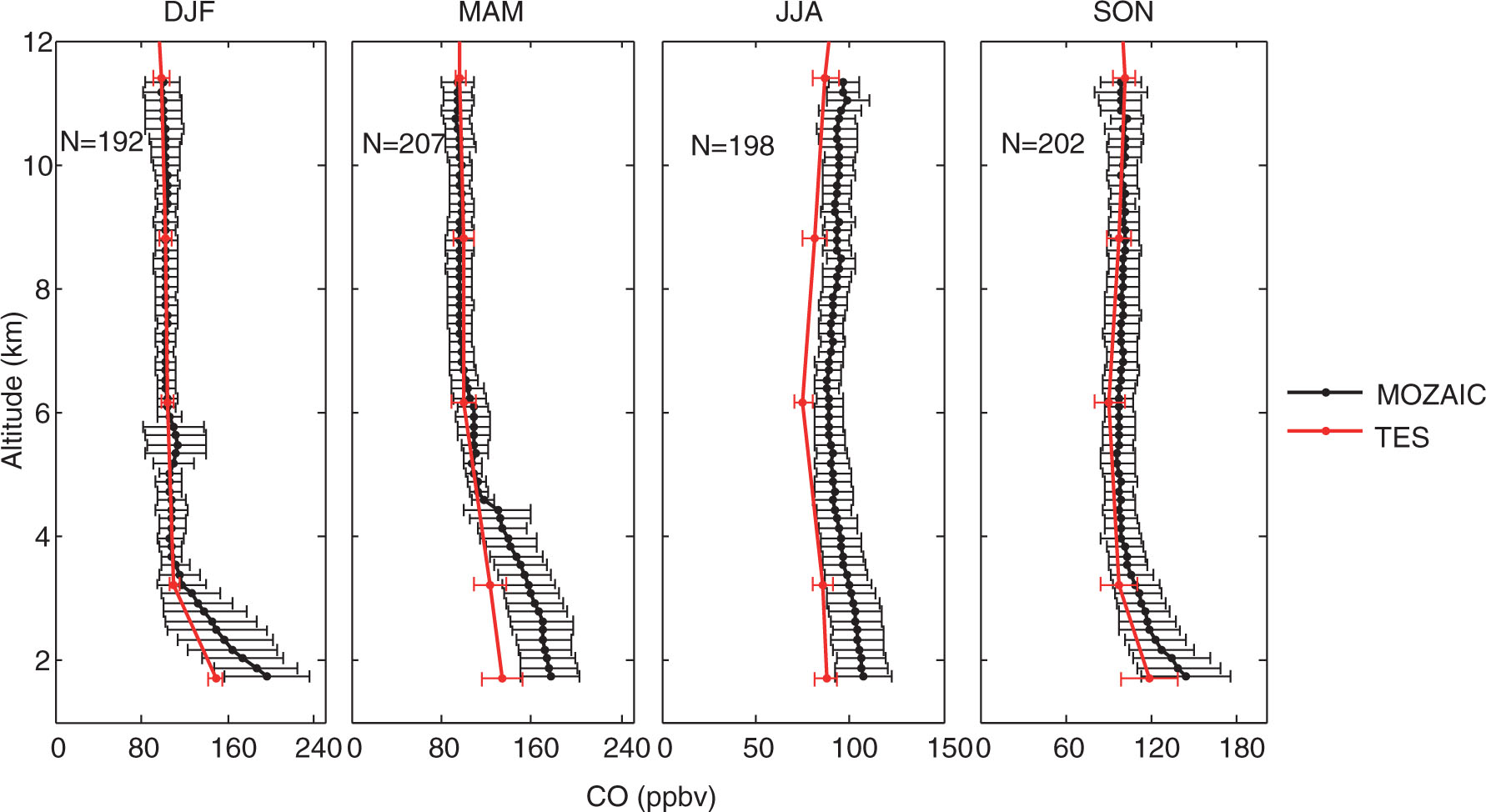
Mean vertical profiles of CO of MOZAIC and TES observations are plotted along with standard deviation for different seasons (DJF, MAM, JJA and SON) during a 5-yr period (2006–2010). N represents the total number of profiles.
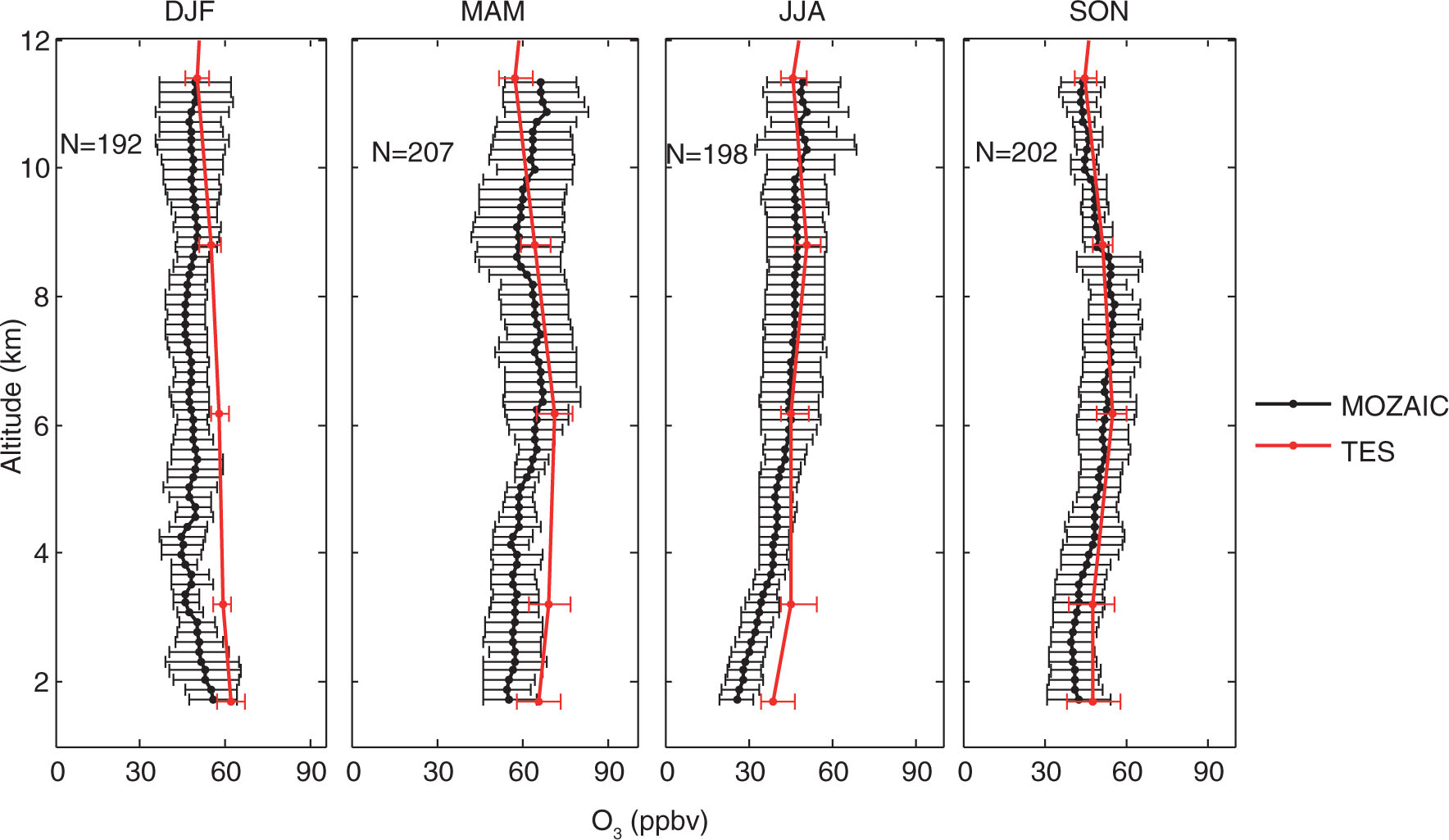
Fig. 2

Mean vertical profiles of O3 of MOZAIC and TES observations are plotted along with standard deviation for different seasons (DJF, MAM, JJA and SON) during a 5-yr period (2006–2010). N represents the total number of profiles.

Table 1. Mean bias between TES and MOZAIC observations for four seasons DJF, MAM, JJA and SON is calculated at different tropospheric altitude regions
Mean bias for CO (ppbv)Mean bias for O3 (ppbv)Time2–8 km8–10 km2–8 km8–10 kmDJF27.90.8−8.6−7.0MAM31.8−2.3−11.0−0.6JJA17.910.1−9.7−3.1SON19.42.8−5.33.3
Fig. 3

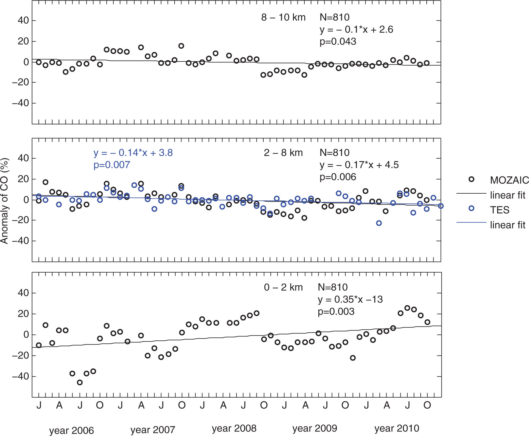
Monthly mean anomalies of CO are shown over Hyderabad in the three tropospheric layers with MOZAIC (0–2, 2–8 and 8–10 km) and TES (2–8 km) observations. N and p represent the total number of MOZAIC profiles and p value, respectively.
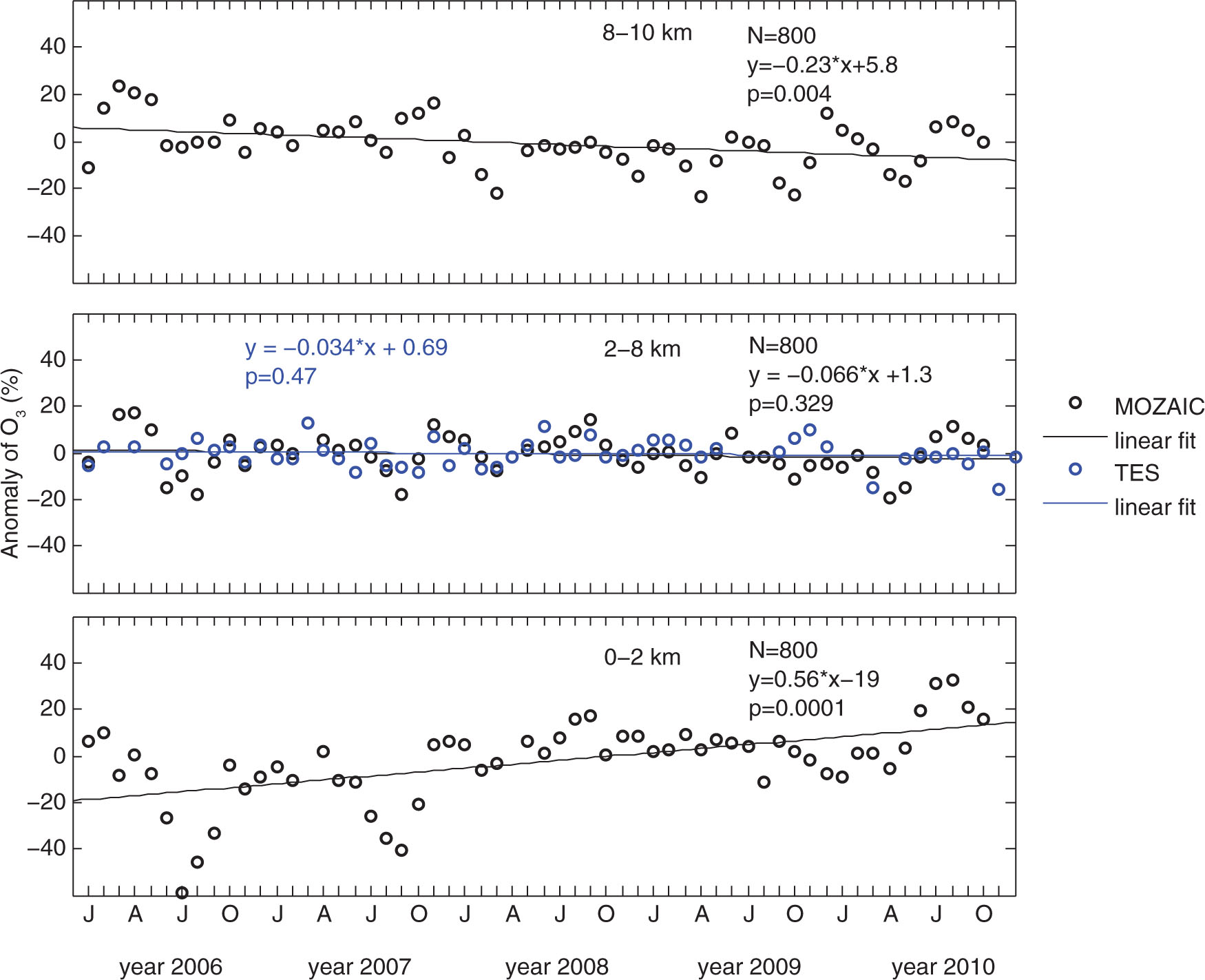
Fig. 4

Monthly mean anomalies of O3 are shown over Hyderabad in the three tropospheric layers with MOZAIC (0–2, 2–8 and 8–10 km) and TES (2–8 km) observations. N and p represents the total number of MOZAIC profiles and p value, respectively.

Table 2. Changes in CO and O3 obtained from MOZAIC observations with respect to the year 2006 in Hyderabad
Hyderabad (17.3°N, 78.4800°E)Tropospheric Layers (km)Changes in CO (% with respect to 2006)Changes in O3 (% with respect to 2006)0–2+4.2±1.3+6.7±1.32–8−2.0 (−1.6)±0.7 (0.4)−0.7 (0.3)±0.7 (0.4)8–10−1.2±0.48−2.7±0.8

[i] Change in CO and O3 with TES observations are shown in 2–8 km layer in bracket along with the MOZAIC observations.

Fig. 5

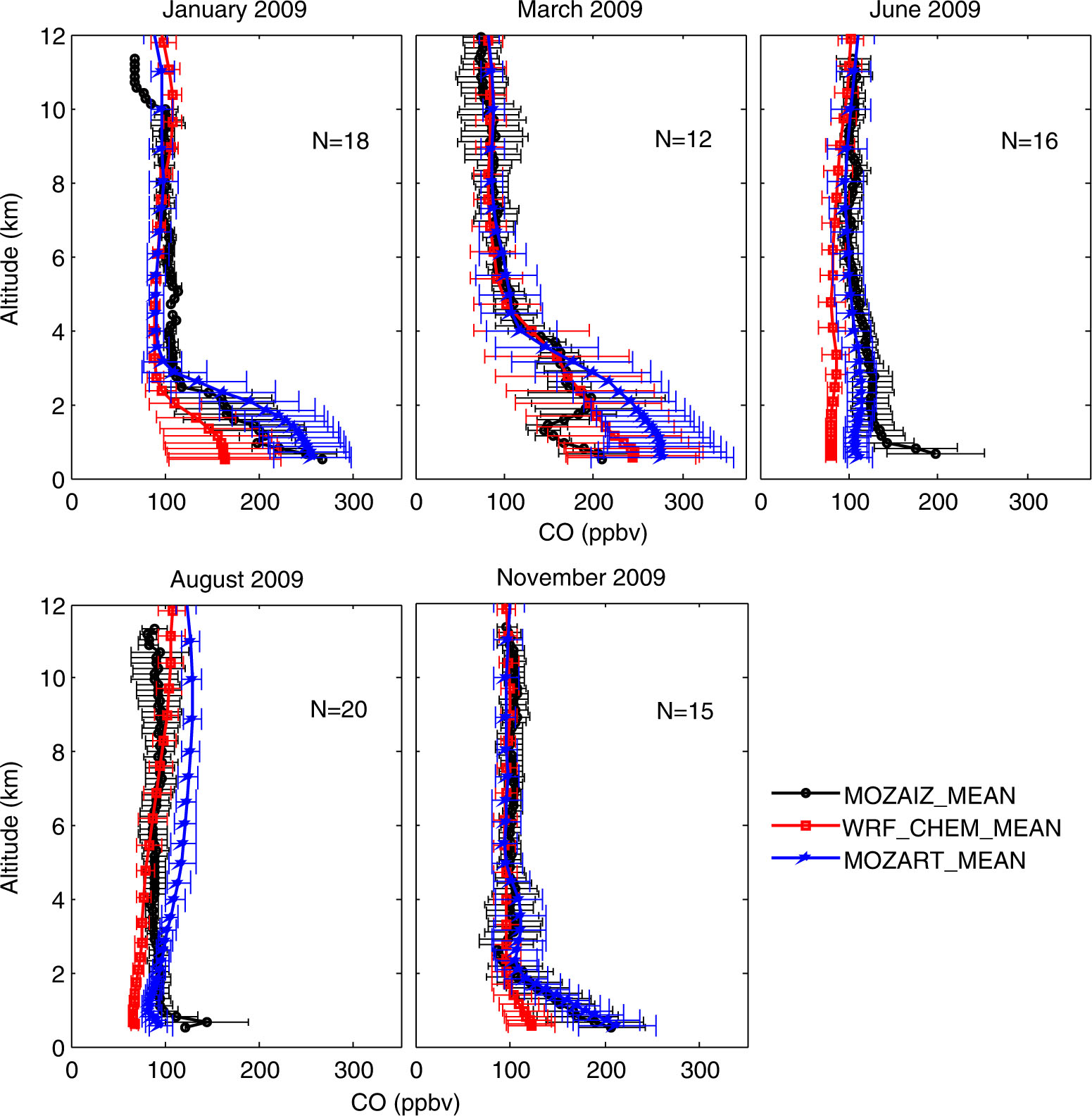
Monthly mean profiles of CO along with standard deviation are plotted for different months of the year 2009 for MOZAIC observations and WRF-Chem and MOZART-4 simulations. N represents the total number of profiles of that particular month.
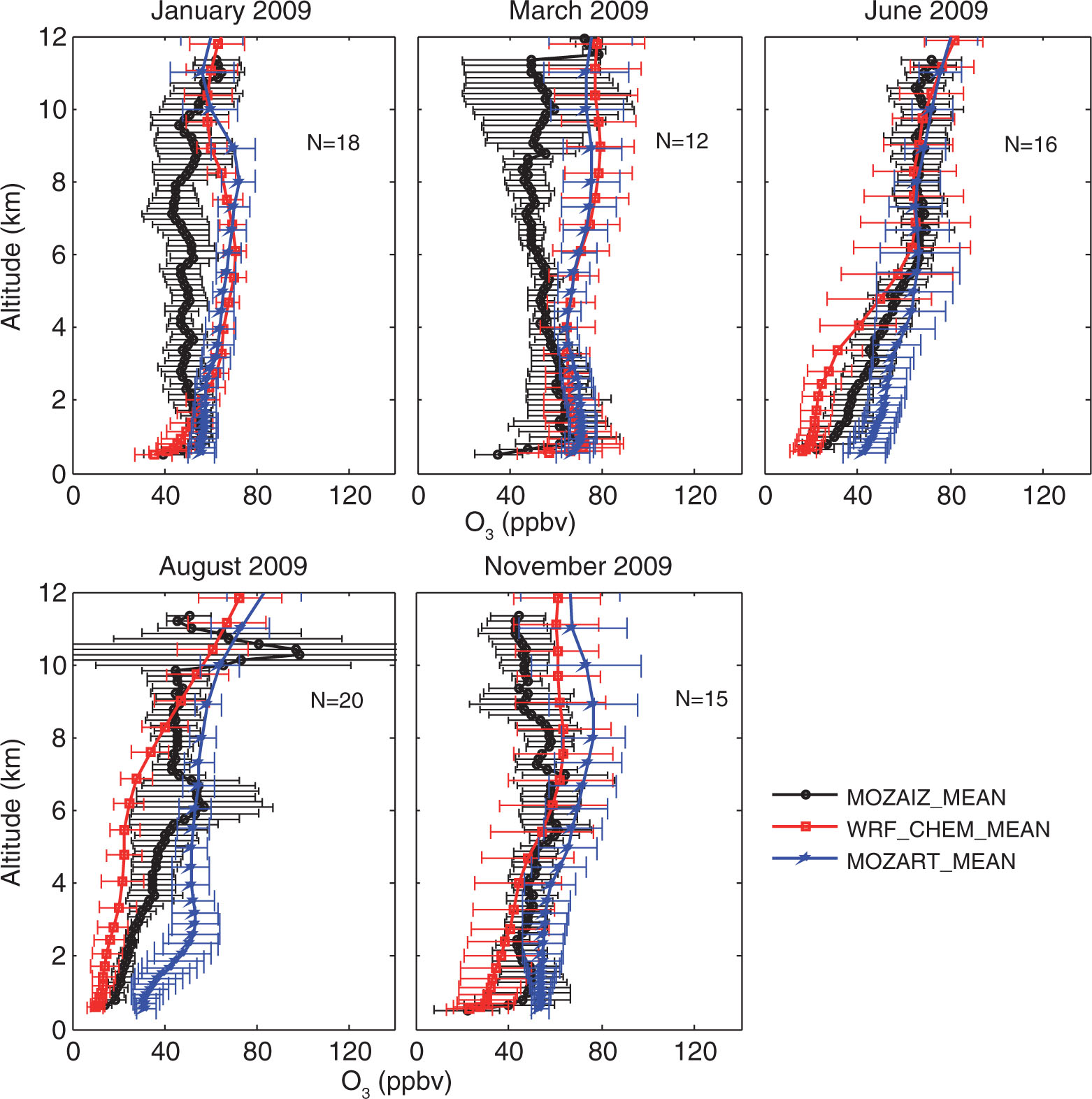
Fig. 6

Monthly mean profiles of O3 along with standard deviation are plotted for different months of the year 2009 for MOZAIC observations and WRF-Chem and MOZART-4 simulations. N represents the total number of profiles of that particular month.

Table 3. Mean bias is calculated for monthly average WRF-Chem and MOZART-4 simulated CO and O3 with respect to MOZAIC observations for different months of the year 2009.
Mean Bias with WRF-Chem (MOZART-4) for CO (ppbv)Time0–2 km2–4 km4–6 km6–8 km8–10 kmJan 200953.6 (−26.9)31.0 (−3.7)7.8 (12.0)7.0 (6.9)−4.4 (2.1)March 2009−49.6 (−71.7)−0.9 (−23.2)5.2 (−1.3)6.8 (0.5)2.4 (−2.2)Jun 200949.3 (23.3)40.7 (11.8)28.8 (6.2)17.4 (1.3)14.1 (5.2)Aug 200943.6 (12.0)16.8 (−11.4)9.0 (−28.2)0.1 (−31.9)−6.5 (−34.4)Nov 200954.5 (−8.6)5.1 (−9.8)4.9 (4.1)5.9 (5.6)5.3 (7.4)Mean Bias with WRF-Chem (MOZART-4) for O3 (ppbv)0–2 km2–4 km4–6 km6–8 km8–10 kmJan 20093.9 (−3.5)−12.5 (−11.5)−19.7 (−17.2)−21.4 (−20.9)−10.9 (−15.7)March 2009−12.1 (−8.3)−5.1 (−7.6)−12.3 (−11.6)−23.9 (−21.9)−27.2 (−21.8)Jun 20097.8 (−11.3)15.0 (−10.7)7.6 (−6.4)2.4 (1.5)1.8 (−0.3)Aug 20095.0 (−11.5)10.0 (−22.9)15.8 (−13.0)20.9 (−2.9)−1.8 (−8.3)Nov 200911.9 (−6.7)6.2 (−8.9)4.6 (−9.9)−2.9 (−15.5)−12.6 (−25.7)
Fig. 7

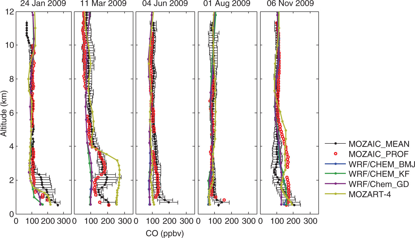
The monthly mean MOZAIC CO profiles (MOZAIC_MEAN) for 5 months of the year 2009 are shown along with the standard deviation. The anomalous profile observed by MOZAIC for a particular month is shown along with the spatially and temporarily collocated profile simulated by WRF-Chem using BMJ, KF and GD convection schemes and MOZART-4 model.

Table 4. Mean bias in O (CO) for the anomalous profiles of the year 2009 is calculated at different layers of the troposphere
24 Jan 2009WRF-ChemAltitude (km)BMJKFGDMOZART-40–2−5.8 (19.8)−5.8 (19.8)−0.2 (5.6)−7.8 (−14.2)2–4−21.8 (19.4)−21.9 (19.4)−22.1 (21.5)−28.6 (17.3)4–6−22.7 (3.0)−22.7 (3.1)−22.3 (3.0)−19.1 (0.4)6–8−5.6 (9.8)−5.6 (9.8)−5.7 (9.5)−6.5 (4.3)8–10−16.3 (3.2)−16.2 (3.2)−17.1 (3.7)−13.9 (10.0)11 March 20090–2−4.1 (37.8)−7.0 (37.7)−6.3 (35.1)−31.4 (−75.3)2–47.8 (77.0)8.5 (76.8)13.1 (70.0)−20.1 (−76.7)4–6−18.7 (13.8)−23.2 (15.1)−22.6 (14.3)−12.2 (−20.3)6–8−44.4 (0.1)−45.4 (0.2)−45.7 (0.1)−22.9 (0.1)8–10−33.7 (−13.4)−33.9 (−13.4)−32.8 (−13.4)−18.2 (−29.7)4 June 20090–25.6 (36.1)7.3 (34.5)4.9 (34.0)−6.9 (20.7)2–45.2 (27.9)6.9 (26.2)7.2 (26.6)−5.1 (19.5)4–60.1 (5.2)−0.4 (5.1)−0.8 (5.1)4.3 (12.0)6–8−12.8 (2.2)−12.3 (2.5)−10.8 (2.7)23.3 (6.1)8–10−20.6 (13.6)−19.3 (14.1)−19.8 (13.3)0.6 (9.5)1 Aug 20090–25.1 (15.7)6.4 (18.9)5.7 (15.3)−2.4 (17.0)2–410.0 (−7.7)12.1 (−2.1)13.5 (−3.1)−9.0 (−8.3)4–616.9 (1.4)14.1 (3.1)19.1 (1.6)10.8 (−10.9)6–838.6 (5.1)31.0 (7.4)31.1 (6.6)32.3 (−23.4)8–1014.0 (5.0)14.3 (6.8)9.6 (2.2)4.9 (−2.8)6 Nov 20090–2−5.3 (16.2)−9.6 (14.2)−11.3 (39.7)−23.6 (16.9)2–46.1 (34.0)8.8 (30.5)2.7 (27.9)−5.4 (11.7)4–6−3.0 (25.1)6.7 (21.5)−4.4 (24.2)8.7 (−23.3)6–8−7.5 (19.5)−8.4 (20.0)−4.4(17.5)11.3 (3.6)8–104.5 (6.5)1.7 (9.8)2.7 (9.4)−17.6 (17.8)
Fig. 9

MOZAIC observed temperature (bottom x-axis labels) and water vapour mixing ratio (top x-axis labels) profiles are plotted along with WRF-Chem simulation corresponding to CO and O3 anomalous profiles.
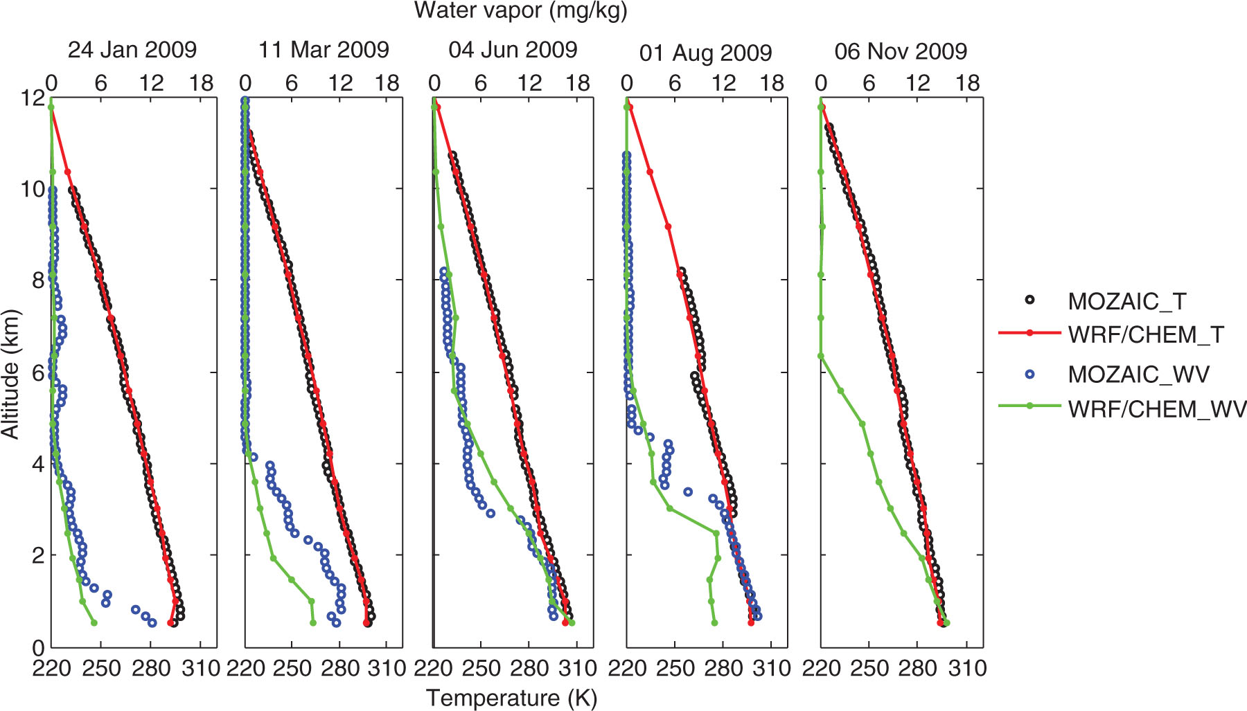
Fig. 10

MOZAIC observed and WRF-Chem simulated wind speed profiles are plotted corresponding to anomalous CO and O3 profiles.
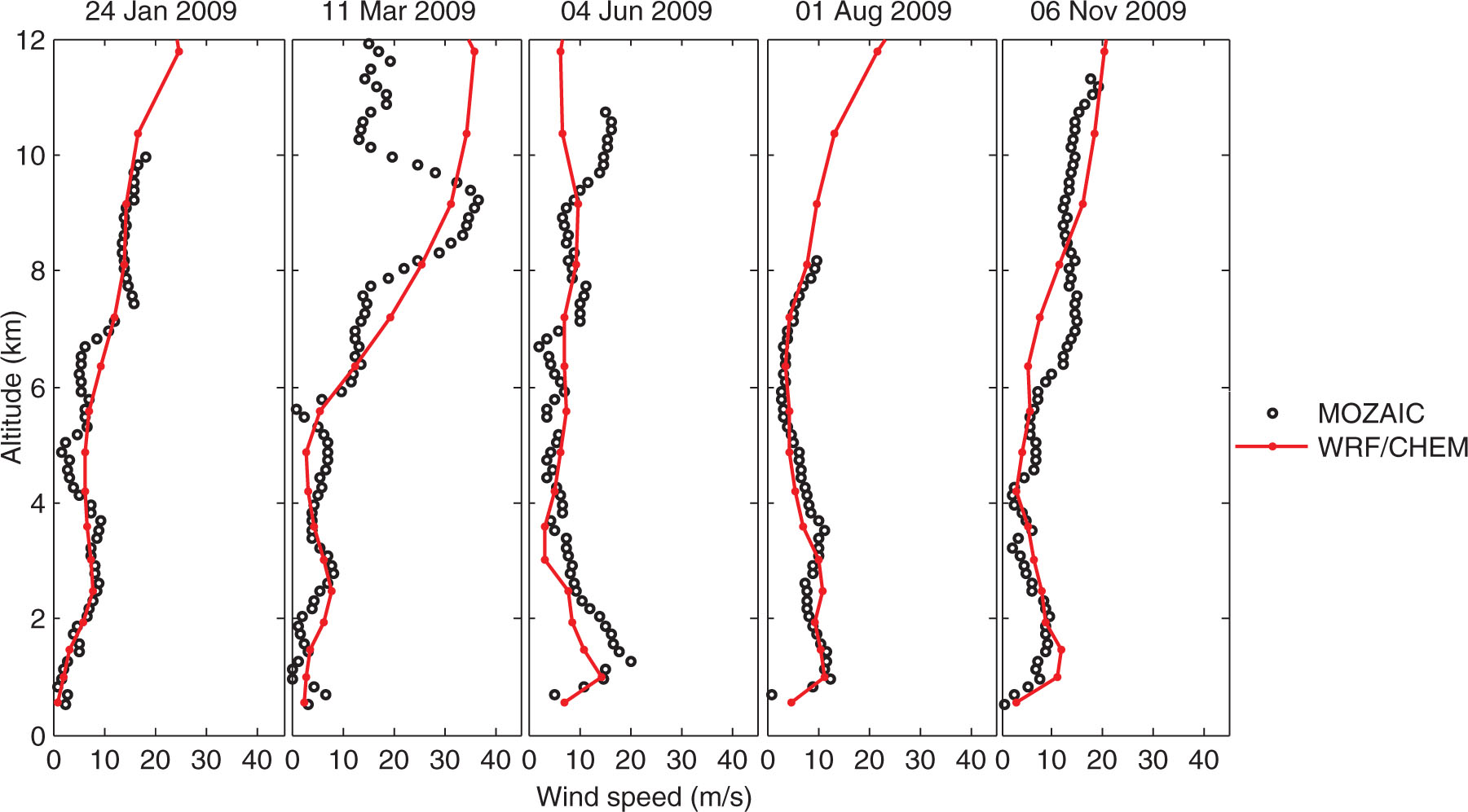
Fig. 11

Wind direction corresponding to anomalous CO and O3 profiles obtained from MOZAIC observation and WRF-Chem simulations are plotted against altitude.
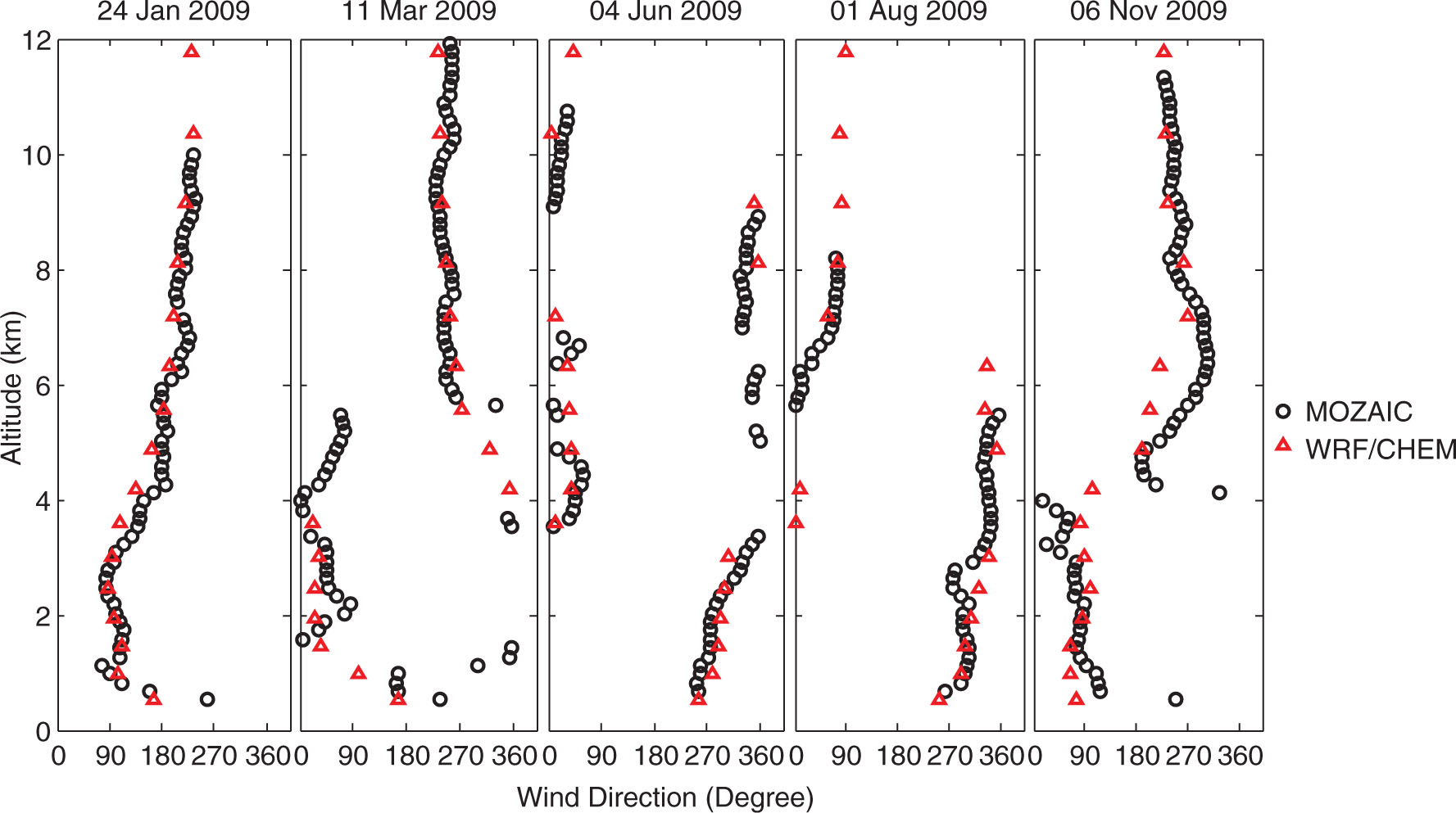
Fig. 12

WRF-Chem winds are plotted overlaid on O3 (ppbv) at 2, 6 and 8 km altitude region at 6, 12 and 18 GMT. The O3 over Hyderabad lies inside the box in the figure.
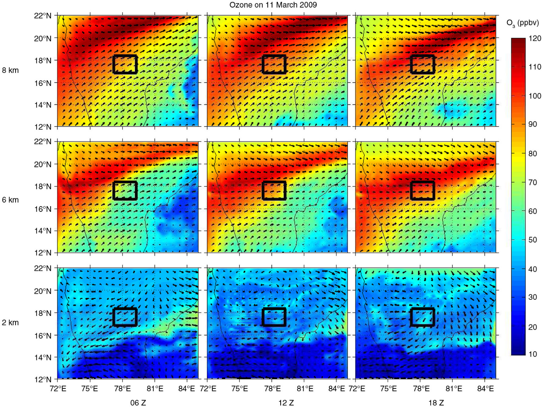
Fig. 13

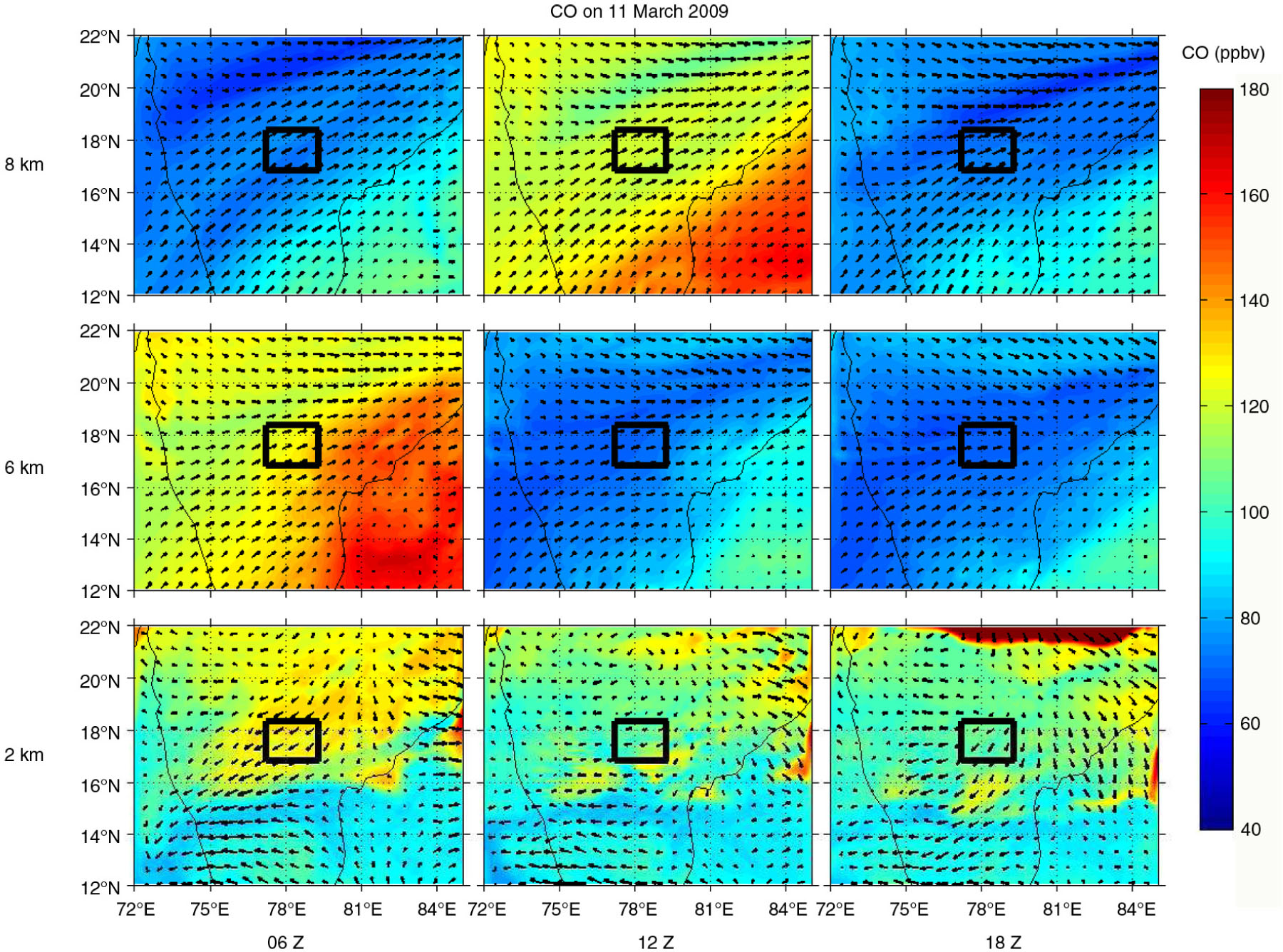
WRF-Chem winds are plotted overlaid on CO (ppbv) at 2, 6 and 8 km altitude regions at 6, 12 and 18 GMT. The CO over Hyderabad lies inside the box in the figure.

Table 5. Mean bias is calculated for WRF-Chem with respect to MOZAIC observations for temperature, water vapour mixing ratio and wind speed at different altitude region
Mean biasTemperature (K)Date0–2 km2–4 km4–6 km6–8 km8–10 km24 Jan 20091.9−0.7−0.60.3−0.211 March 20090.40.0−1.2−0.20.64 June 20090.50.60.51.50.01 Aug 20090.51.2−0.92.00.46 Nov 20091.4−0.7−0.1−0.11.6Water vapour mixing ratio (mg/kg)24 Jan 20092.80.80.50.00.011 March 20094.63.00.10.00.04 June 20093.03.10.10.10.11 Aug 20090.1−2.0−0.4−0.5−0.3Wind speed (m/s)24 Jan 20090.61.1−2.3−1.90.411 March 2009−1.6−0.50.8−2.31.54 June 20093.22.7−1.60.3−1.41 Aug 20090.20.00.90.30.86 Nov 2009−2.0−1.40.86.7−0.4
Fig. 8

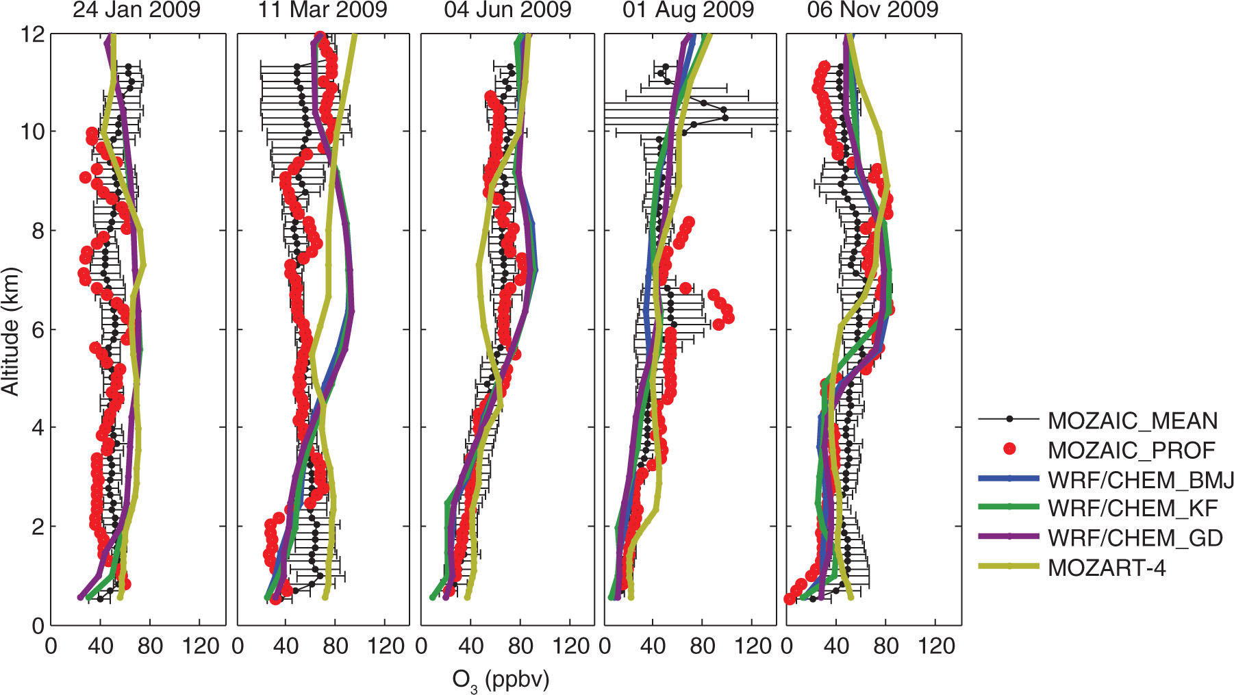
The monthly mean MOZAIC O3 profiles (MOZAIC_MEAN) for 5 months of the year 2009 are shown along with the standard deviation. The anomalous profile observed by MOZAIC for a particular month is shown along with the spatially and temporarily collocated profile simulated by WRF-Chem using BMJ, KF and GD convection schemes and MOZART-4 model.

Language: English
Page range: 30545 - 30545
Submitted on: Nov 27, 2015
Accepted on: Apr 13, 2016
Published on: Jan 1, 2016
Published by: Stockholm University Press
In partnership with: Paradigm Publishing Services
Keywords:

© 2016 Varun Sheel, Jagat Singh Heet Bisht, Lokesh Sahu, Valérie Thouret, published by Stockholm University Press
This work is licensed under the Creative Commons Attribution 4.0 License.