
1. Introduction
In 1961, Craig published his findings that the stable hydrogen and oxygen isotopic compositions of fresh waters are highly correlated; according to the ‘global meteoric water line’, he determined them as
where SMOW is the Standard Mean Ocean Water—Vienna Standard Mean Ocean Water (VSMOW; Gonfiantini, 1978) did not yet exist. Three decades later this relationship in precipitation was refined by Rozanski et al. (1993) at the International Atomic Energy Agency (IAEA):
where the factor of 10−3 has been added so that the equation is in accord with the International System of Units [Bureau International des Poids et Mesures (BIPM), 2006; Coplen, 2011]. Although the evolution of δ 2HVSMOW and δ 18OVSMOW of precipitation begins with evaporation of water from the oceans, their relationship arises primarily from equilibrium fractionation of heavier and lighter isotopes of hydrogen and oxygen during condensation as a tropospheric vapour mass follows a trajectory to higher latitudes and over continents, a process called ‘rainout’ (Dansgaard, 1964; Rozanski et al., 1993; Clark and Fritz, 1997). Condensation is produced through cooling of an air mass. Cooling occurs by adiabatic expansion as an air mass ascends or by radiative heat loss. It is Rayleigh distillation (Rayleigh, 1896) during rainout of precipitation that gives rise to the global meteoric water line (Dansgaard, 1964):
where R 0 and R are the vapour's initial isotope ratio and isotope ratio after rainout, respectively. The quantity f is the residual fraction of vapour in the air mass, and α is the equilibrium isotopic fractionation factor between vapour and liquid water at the in-cloud temperature.
Dansgaard (1964) first suggested the use of the intercept in the Craig (1961) relation above to characterise a precipitation sample. The quantity deuterium excess, d E, where superscript E indicates an excess quantity (IUPAC Physical Chemistry Division, 2007) is defined by the relation
Regionally, d E varies due to variations in humidity, wind speed and sea-surface temperature during primary evaporation (Rozanski et al., 1993; Clark and Fritz, 1997). Although the mean global value of d E is ~10 ‰, low d E values correlate with higher values of relative humidity during primary evaporation (Rozanski et al., 1993).
Because temperature is the primary driver of rainout, δ 2HVSMOW and δ 18OVSMOW values of mean annual precipitation are strongly correlated with surface temperature (not in-cloud temperature), as was first shown by Dansgaard (1964), who found:
where T annual is the annual mean air temperature and where SMOW has been replaced by VSMOW, which is in use today. On average, a 10 ‰ decrease in δ 2HVSMOW of precipitation corresponds to a decrease in average temperature of about 1.4–2.1 °C (Dansgaard, 1964; Rozanski et al., 1993), and a concordant decrease is observed for δ 18OVSMOW values. Because mean annual temperature decreases with increasing latitude, this temperature effect gives rise to the well-known latitude effect in which higher latitudes have lower δ 2HVSMOW and δ 18OVSMOW values of mean annual precipitation (Dansgaard, 1964; Rozanski et al., 1993). Similarly, transit of vapour masses across continents with their decreasing temperatures owing to topographic increases gives rise to the well-known continental effect in which lower δ 2HVSMOW and δ 18OVSMOW values of mean annual precipitation are observed on average with increasing distance from an ocean–continent boundary (Dansgaard, 1964; Rozanski et al., 1993). Variations of δ 2HVSMOW and δ 18OVSMOW of precipitation are observed with seasonal variations in temperature, giving rise to the seasonal effect, and this seasonal effect is amplified with increasing continentality of a collection site (Clark and Fritz, 1997). On a local basis, increases in topographic relief can promote adiabatic cooling as a vapour mass ascends over the landscape, with resulting orographic precipitation and concordant rainout, giving rise to the well-known altitude effect. Variation in δ 2HVSMOW and δ 18OVSMOW of precipitation with altitude of −1 to −4 ‰ per 100 m and −0.15 to −0.5 ‰ per 100 m, respectively, have been published for the altitude effect (Clark and Fritz, 1997 and references therein).
Measurements of δ 2HVSMOW and δ 18OVSMOW of precipitation provide a natural tracer of atmospheric processes (Gedzelman and Lawrence et al., 1990; Scholl et al., 2007; Smith and Evans, 2007). Organised ascent is often associated with specific regions within extratropical cyclones, including storms that impact the western coast of North America during the winter wet season. Studies using meteorological arrays have provided insights into precipitation-generating processes (Neiman et al., 2002, 2004; Kingsmill et al., 2006; Ralph et al., 2006, 2013a; Smith et al., 2010) and precipitation characteristics during such storm events (White et al., 2003; Martner et al., 2008). These meteorological findings helped shape the present work by revealing processes that would be expected to impose distinct isotopic signatures on the resulting precipitation. Notably, precipitation with a radar brightband (BB) signature starts as ice above the BB and melts into rain as it falls through the BB altitude. Because such precipitation occurs initially at higher (and much colder) altitudes, it would be expected to have an isotopic composition depleted in 2H and 18O (Dansgaard, 1953) and rainout is relatively high. In contrast, a shallow rainfall process occurring without a BB, that is, non-brightband (NBB) rain, forms primarily at low altitudes (White et al., 2003; Neiman et al., 2005; Martner et al., 2008) and is expected to exhibit an isotopic composition consistent with a relatively warm marine source (more enriched in 2H and 18O), and rainout is substantially lower.
Many of the events in this study are atmospheric rivers (ARs), which are characterised by strong horizontal water-vapour fluxes concentrated in a narrow band in the lower troposphere immediately ahead of the polar cold fronts. ARs are also associated with winter storms formed over the oceans at midlatitudes (Zhu and Newell, 1998; Ralph et al., 2004). They are readily identifiable in Special Sensor Microwave/Imager (SSM/I) satellite imagery as long, narrow plumes of enhanced integrated water vapour (Hollinger et al., 1990). They often produce heavy coastal rainfall and flooding along the US West Coast (Ralph et al., 2006). During landfalling Pacific winter storms, ARs provide a focused moisture source, leading to orographic rainfall enhancement in the coastal mountains (Ralph et al., 2004; Bao et al., 2006).
With an automated precipitation collector, Coplen et al. (2008) observed a substantial decrease in stable hydrogen isotopic composition (δ 2HVSMOW) in a landfalling Pacific storm along the California coast at Cazadero (CZD; location shown in Fig. 1), on 21 March 2005 (Fig. 2). The δ 2HVSMOW of precipitation decreased by 51 ‰ over a 60-min period as precipitation generation transitioned from a shallow to a much deeper cloud layer, in accord with synoptic-scale ascent and deep ‘seeder–feeder’ precipitation (Bergeron, 1935; Findeisen, 1938). The seeder–feeder mechanism is (Meteorology Glossary, 2015) ‘Orographic precipitation-enhancement mechanism, in which precipitation from an upper-level precipitating cloud (seeder) falls through a lower-level orographic stratus cloud (feeder) capping a hill or small mountain. Precipitation droplets or ice particles fall from the higher seeder cloud and collect cloud water as they pass through the lower feeder cloud by collision and coalescence or accretion, thus producing greater precipitation on the hill under the cap cloud than on the nearby flat land. The effectiveness of the process depends on sufficiently strong low-level moist flow to maintain the cloud water content in the orographic feeder cloud and the continuing availability of precipitation particles from the seeder cloud’. Following a 3-h period of relatively constant, low δ 2HVSMOW values of precipitation corresponding to higher rainout, the δ 2HVSMOW increased by a remarkable 58 ‰ during the next 3 h corresponding to lower rainout. Zones of distinct isotopic behaviour are identified by Roman numerals in Fig. 2d: I, virga and initial pre-cold frontal precipitation as atmospheric column saturates; II, transitional mixing of I and III; III, precipitation from deep, cold cloud layer via the seeder–feeder mechanism; IV, transitional mixing between III and V; V, shallow, locally generated orographic rain; VI, light rainfall with passage of cold front. Yoshimura et al. (2010) used the isotope-abundance measurements of the March 2005 storm event (Coplen et al., 2008) in a regional model for simulations of the March 2005 storm, and their conclusions are discussed in Section 4.9.
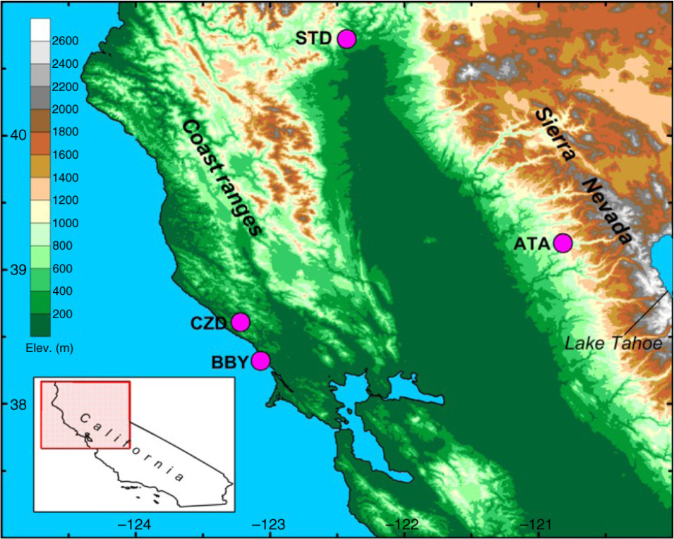
Fig. 1
Location of data collection sites in this investigation.
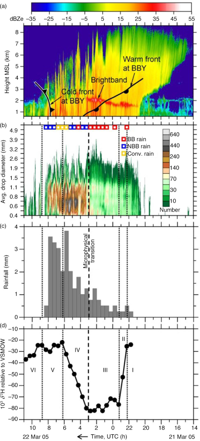
Fig. 2
Observations at Cazadero, CA (CZD) on 21–22 March 2005 (from Coplen et al., 2008). Time increases from right to left. (a) Time–height section of equivalent radar reflectivity factor (dBZe; see colour scale). (b) Contoured drop-size distributions of rainfall at the surface as a function of time and diameter (see colour scale). Open squares indicate objective categorisation of the rainfall occurring during selected half-hour periods; BB (red), rain with a radar brightband signature; NBB (blue), rain without a radar brightband signature; Conv. (yellow), convection rain. (c) Histogram of hourly rainfall (mm). (d) Time series of stable hydrogen isotopic composition of 30-min, time-integrated precipitation samples. A primary change in precipitation microphysical properties is marked by the vertical dashed lines in Fig. 2b–d. Zones of distinct isotope behaviour are enclosed by the vertical lines and labelled with Roman numerals in (d): I, pre-cold frontal precipitation of marine air; II, transitional mixing of I and III; III, precipitation from deep, cold cloud layer via the seeder–feeder mechanism; IV, transitional mixing between III and V; V, shallow, locally generated orographic rain; VI, light rainfall with passage of cold front.
Muller et al. (2015) measured δ 2HVSMOW of a total of 242 sequentially collected rainfall samples from 16 precipitation events collected in Birmingham, United Kingdom between 26 April 2005 and 11 October 2006 during different seasons and over a range of synoptic conditions with an innovatively modified, tipping-bucket rain gauge. They also used a vertically pointing micro rain radar having frequency-modulated, continuous-wave Doppler radars operating at 24 GHz, which enabled high-resolution determination of microphysical characteristics (e.g. rain rate, fall velocity and drop-size distributions). Their results indicated that some midlatitude events show substantial variations in δ 2HVSMOW of rainfall during an event, and they observed a maximum variation in δ 2HVSMOW of rainfall of 55.4 ‰ during a 5 October 2006 event.
One question posed in this paper is whether the decrease in δ 2HVSMOW of precipitation observed in the single case study analysed by Coplen et al. (2008) is unique or more common. With landfall of extratropical cyclones, what insights might stable-isotope measurements of rainfall provide into precipitation-generating processes? If these variations in isotopic composition are common features, they might be used by isotope hydrologists to investigate hydrograph separation. Because the Coplen et al. (2008) only scratched the surface and motivated a much larger data collection and analysis effort, automated precipitation collectors were located at four spatially diverse, California sites during selected periods between 2007 and 2011 to obtain precipitation samples with landfall of extratropical cyclones.
2. Observing systems
This study analyses data collected from unique meteorological instrumentation from 2000 to 2011 deployed at four geographically diverse locations in northern California (see Fig. 1 and Table 1 for locations and elevations): Bodega Bay (BBY), CZD, Alta (ATA) and Shasta Dam (STD). The deployments supported the National Oceanic and Atmospheric Administration's (NOAA) Hydrometeorological Testbed programme (Ralph et al., 2005, 2013b; White, 2012) and the California Energy Commission's CalWater Project (www.esrl.noaa.gov/psd/calwater; Ault et al., 2011). Details of the instrumentation are described below.
The U.S. Geological Survey deployed a novel rainfall isotope collector at each of the four observing sites. The collectors obtained precipitation samples at an unprecedented temporal resolution of 30 min. A complete description of these collectors and associated data analysis techniques are provided in Section 3. Each precipitation collector was accompanied by a collocated 10-m tower that measured surface meteorological parameters (i.e. temperature, relative humidity, surface pressure, wind velocity, and precipitation) every 2 min.
NOAA's Physical Sciences Division (NOAA/PSD) deployed three different types of radars. Vertically pointing S-band precipitation profiling radars (S-PROF) were stationed at CZD and ATA. The S-PROFs operated with a frequency of 2875 MHz (i.e. 10-cm wavelength) and with an extended dynamic range of nearly 100 dB (White et al., 2000). They provided high time-resolution profiles of power return and vertical radial velocity from ~250 m MSL up to 8 km MSL. The S-PROF data were used to classify precipitation into BB, NBB and convective (Conv) precipitation via the rainfall process partition analysis technique (White et al., 2003). A frequency-modulated constant-wavelength S-band snow-level radar was deployed at STD and provided power and radial velocity data similar to that of the S-PROFs, but with 40-m vertical resolution and 36-s temporal resolution. A 915-MHz wind profiler at BBY provided hourly averaged vertical profiles of horizontal wind velocity from ~0.1 to 4.0 km above ground with ~100-m vertical resolution and ~1 m s−1 accuracy (Carter et al., 1995). For all the radars described above, the height of the radar BB, generated by melting precipitation (e.g. Battan, 1973), was obtained hourly using the objective BB detection method of White et al. (2002).
3. Precipitation isotope collectors and isotope analysis
This study required sequential collection of many time-integrated precipitation samples over short (30-min) intervals to capture quantitatively rapid changes in δ 2HVSMOW and δ 18OVSMOW of precipitation (rain, snow, graupel and hail). An automated sequential time-integrated collector of precipitation (Coplen, 2010, US patent no. 7687028; see also Supplementary File of Coplen et al., 2008) for obtaining 96 sequential 15-mL samples was constructed and installed at CZD between January and March of 2005. Four automated collectors were installed at ATA, BBY, CZD and STD during selected periods between 2007 and 2011 (all four sites are listed in Table 1). Upon notification of the approach of a landfalling storm by NOAA weather forecasters, the collectors were started either by landline phone, delayed actuation or manual initiation.
Table 1. Sample collection sites in California
Since invention of the automated collector, laser absorption spectrometers have been developed and advocated for analysis of precipitation samples in the field (Berman et al., 2009; Munksgaard et al., 2011). These instruments have the following deficiencies:
They do not have delayed or remote start capability (for periods of weeks to months) using a cell phone or landline phone.
They are not able to collect and measure samples below freezing, such as snow and hail.
They are not able to collect time-integrated samples, such as 30-min integrated rainfall samples. Rather, they collect and measure instantaneous or intermittently collected samples.
Precipitation samples were analysed for their isotopic composition at the U.S. Geological Survey's Reston Stable Isotope Laboratory (www.isotopes.usgs.gov/). The isotopic composition of hydrogen is denoted herein by the quantity δ 2HVSMOW, which is defined by the relation (Coplen, 2011)
where R(2H/1H)P is the ratio N(2H)P/N(1H)P, and N(2H)P and N(1H)P are the numbers of the two isotopes of hydrogen, 2H and 1H, respectively, in a sample P (Coplen, 2011). Commonly, an extraneous numerical factor of 1000 is added to this definition. However, to be consistent with the Système International d'Unités, the SI (known in English as the International System of Units), which is published by the BIPM, the factor 1000 should not appear in this equation in order that this equation is written as a quantity equation and not as a numeric value equation (BIPM, 2006; Coplen, 2011). In a similar manner, R(2H/1H)VSMOW is the equivalent hydrogen-isotope ratio in the international isotopic measurement standard VSMOW. Similarly, the isotopic composition of oxygen is denoted by the quantity δ 18OVSMOW, which is defined in an equivalent manner by the relation
An isotope-delta measurement is a differential measurement and can be negative or positive. The more positive the isotope delta, the higher the fraction of the heavy isotope (2H and 18O), and the more negative the isotope delta, the lower the fraction of the heavy isotope in the sample.
The isotope scales δ 2HVSMOW and δ 18OVSMOW are normalised such that δ 2HVSMOW and δ 18OVSMOW values of the international measurement Standard Light Antarctic Precipitation reference water are −428 and −55.5 ‰, respectively (Gonfiantini, 1978). Measurements of δ 2HVSMOW were performed by gaseous hydrogen–water equilibration with a platinum catalyst (Coplen et al., 1991), followed by dual-inlet isotope-ratio mass spectrometry (Révész and Coplen, 2008a). Measurements of δ 18OVSMOW of water were performed by carbon dioxide–water equilibration, followed by dual-inlet isotope-ratio mass spectrometry (Révész and Coplen, 2008b). The 1 - σ uncertainty of δ 2HVSMOW measurements is ±1 ‰ and that of δ 18OVSMOW measurements is ±0.1 ‰.
4. Results and discussion
In this study, during the period 2005–2011, 1398 samples were analysed for δ 2HVSMOW: 866 from CZD, 315 from BBY, 195 from ATA and 22 from STD. Because some samples were small and were analysed first for their δ 2HVSMOW value, only 1384 samples could be analysed for their δ 18OVSMOW values. All these measurement results are presented in the Supplementary File, and most of these data are shown in figures associated with this document. All collection times in figures and text, and in the Supplementary File, are mean collections times of 30-min integrated precipitation samples.
4.1. Correlation between δ 2HVSMOW and δ 18OVSMOW values
The correlation between δ 2HVSMOW and δ 18OVSMOW measurements of all samples from each of the four sites is shown in Fig. 3. The equations of the least-squares regressions are:
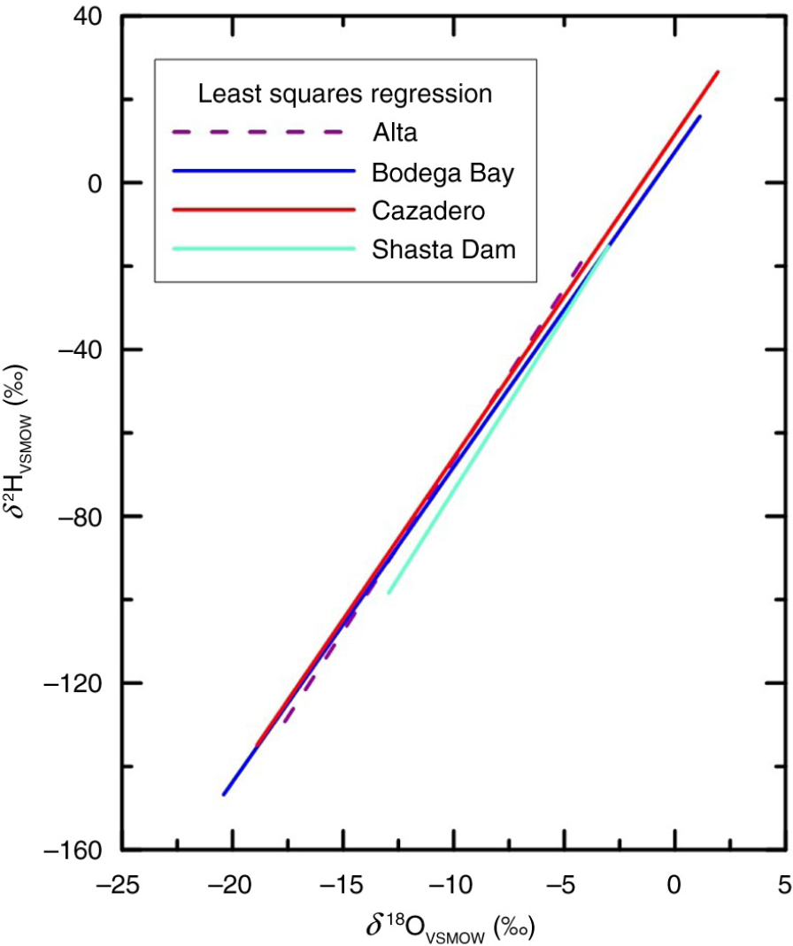
Fig. 3
Crossplot of δ 2HVSMOW and δ 18OVSMOW measurements from the four sites in this study.
These compare well with the global meteoric water line of Rozanski et al. (1993) in eq. (2). The Supplementary File contains δ 2HVSMOW and δ 18OVSMOW crossplots for the 43 events in this study.
The deuterium excess values, d E, defined in eq. (4), are provided in the Supplementary File for 1384 precipitation samples, and the mean values at each site are:
The mean value of d E of 10.2 ‰ for BBY is in agreement with that of California river waters, but mean d E values at CZD and ATA are ~4 ‰ higher than expected based on measurements of California river waters (Kendall and Coplen, 2001). The variability in d E values decreases inland from the Pacific Ocean. There is substantial variation in some samples. For example, the d E values for ATA range from −1.5 to +19.0 ‰. Those for BBY range from −21.4 to +22.7 ‰, and those for CZD range from −22.9 to +23.0 ‰. An important use of d E values is to quantify kinetic isotopic fractionation of falling raindrops, which is discussed in Section 4.9.
4.2. Magnitude and duration of δ 2HVSMOW variations of precipitation
During the event shown in Fig. 2, substantial rainfall began about 2115 UTC 21 March and continued until about 0830 UTC 22 March 2005. During Period II, the precipitation source transitioned rapidly from a predominantly warm (shallow) region to a much colder, more-elevated one with higher rainout owing to a deep cloud layer via a seeder–feeder mechanism. Coplen et al. (2008) were able to apply the numerical closed-system, Rayleigh-based model [eq. (3)] of Gonfiantini and Gherardi (2006), and Coplen et al. (2008) calculated an in-cloud precipitation temperature of −4.2 °C and an amount fraction of water precipitated from the deep cloud layer during rainout of 0.60 [1 – f in eq. (3)] from model inputs of δ 2HVSMOW of Period III precipitation=−78 ‰ and δ 2HVSMOW of initial Pacific Ocean precipitation (~15 °C)=−11.6 ‰. Thus, during Periods II and III the site was under the influence of a cold, deep cloud layer from which 60 % of its original water vapour had precipitated. The opposing mode was observed by Coplen et al. (2008) during Periods IV and V in Fig. 2. Beginning at 0300 UTC 22 March 2005, precipitation transitioned to much shallower, locally generated orographic precipitation as the δ 2HVSMOW of rainfall increased to a maximum value of −22.0 ‰ at 6 UTC. For this much lower rainout source, using the model of Gonfiantini and Gherardi (2006), Coplen et al. (2008) calculated an in-cloud precipitation temperature of 10.1 °C and an amount fraction of water precipitated from the warmer cloud of 0.19. Between 2115 UTC 21 March and 0830 UTC 22 March 2005, the site was under the influence of two substantially different precipitation sources. Between 2115 UTC 21 March and 0300 UTC 22 March 2005, the amount fraction of water remaining in the cold water-vapour source was 0.40, whereas after 0300 UTC the fraction of water remaining in the warmer water-vapour source was 0.81.
Based on the observations of Coplen et al. (2008), shown in Fig. 2, intervals of contrasting rainout might be expected during landfall of other extratropical cyclones. To evaluate this hypothesis, we measured δ 2HVSMOW and δ 18OVSMOW values of precipitation collected at periods of 30 min during landfall of extratropical cyclones at four sites (ATA, BBY, CZD and STD) for 43 events during the period 2005–2011 (Table 2). The equivalent radar reflectivity factor (or hourly wind profiles at BBY), δ 2HVSMOW time series of precipitation, and histogram of rainfall are shown for these 43 events in figures herein, including the figures in the Section 7. As shown in Fig. 2, rainfall during the event at CZD beginning at 2200 UTC 21 March 2005 can be categorised as (1) rain with a radar BB signature (open red squares), (2) rain without a BB signature (NBB; open blue squares), (3) convection rain (open yellow-gold squares) or (4) light rain (<1 mm h−1) or frozen precipitation that could not be categorised or periods of no rain or virga (no open square). In an identical manner, these categorisation data are plotted on figures for 25 CZD events and 1 ATA event for which categorisation data at 30-min intervals exist (S-PROF real-time images and selected real-time data are available at ftp://ftp1.esrl.noaa.gov/psd2/data/real time). No 30-min categorisation data are available for BBY or STD.
Table 2. Decreases and increases in δ 2HVSMOW of precipitation in this study
Decreases in δ 2HVSMOW of precipitation were identified in 82 intervals of these 43 events, ranging from 7.3 to 100.5 ‰ (Table 2) with more than half of the δ 2HVSMOW decreases ranging between 10 and 40 ‰ (Fig. 4a). The average δ 2HVSMOW decrease was 34.6 ‰, with a remarkable 100.5 ‰ decrease observed for a 21 January 2010 event at BBY (Table 2). The maximum δ 2HVSMOW decrease at CZD was 95.7 ‰ for a 6 March 2011 event, that for ATA was 91.4 ‰ for a 9 February 2007 event, and that for STD was 80.3 ‰ for a 6 March 2011 event (Table 2). These results confirm that the δ 2HVSMOW decrease in precipitation of 51.3 ‰ observed by Coplen et al. (2008) over a 60-min period from landfall of an extratropical cyclone at CZD on 21 March 2005 (Fig. 2) is not unique, but is a more common feature of these winter storms.
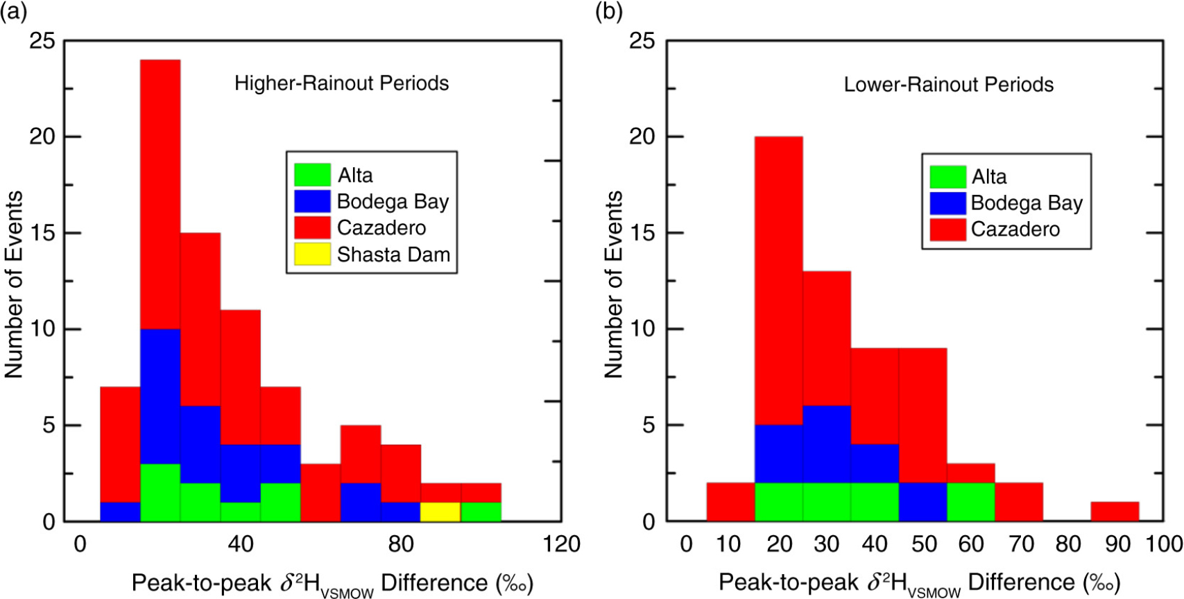
Fig. 4
Histograms of peak-to-peak δ 2HVSMOW differences for sites in this study: (a) peak-to-peak δ 2HVSMOW differences for higher rainout periods and (b) peak-to-peak δ 2HVSMOW differences for lower rainout periods. Data are from Table 2.
Increases in δ 2HVSMOW of precipitation, corresponding to transition to a warmer precipitation source having a substantially higher amount fraction of water vapour (lower rainout), were identified during 61 periods, and they ranged from 4.3 to 82.3 ‰ (Table 2) with approximately half of the δ 2HVSMOW increases ranging between 10 and 40 ‰ (Fig. 4b). The average δ 2HVSMOW increase was 29.3 ‰, with a maximum 82.3 ‰ increase observed for a 10 February 2007 event at CZD (Table 2). The maximum δ 2HVSMOW increase at BBY was 47.6 ‰ for a 23 February 2010 event and that for ATA was 59.7 ‰ for a 9 February 2007 event (Table 2).
4.3. Algorithmic-isotopic categorisation of rainfall into rainout mode
As shown in Section 4.2 and Fig. 2, two precipitation sources with their contrasting rainouts can often be distinguished by precipitation with landfall of extratropical cyclones. The first is a precipitation source having higher rainout (deep, cold clouds) that correlates with decreasing or low δ 2HVSMOW values. In Fig. 2, periods of decreasing or low δ 2HVSMOW values of rain are identified as Periods II and III, and we have added pink panels to figures herein to identify such periods of higher rainout having decreasing or low δ 2HVSMOW values of precipitation, and these panels are labelled ‘HR’ for higher rainout herein. The second mode is from a source having substantially lower rainout (shallow, warm clouds) that correlates with increasing or higher δ 2HVSMOW values. In Fig. 2, periods of lower rainout having increasing or high δ 2HVSMOW values of rain are identified as Periods IV and V, and we have added blue panels to figures herein to identify such periods of lower rainout, and these panels are labelled ‘LR’ for lower rainout herein. For the 21–22 March 2005 event shown in Fig. 2, the pink panel and blue panel are shown in Fig. A5. We term this method to categorise the two rainout modes observed herein as the algorithmic-isotopic categorisation of rainfall. The rules or criteria used to distinguish these two categories of rainout are:
HR (higher rainout, pink panels) periods begin with a rainfall rate of 0.6 mm h−1 or higher and a change in δ 2HVSMOW with time of at least −5 ‰ h−1. The HR period can begin as soon as the rainfall rate achieves a value of 0.6 mm h−1 as shown in Fig. A35 for the 21 January 2010 event at BBY.
During an HR period, small variations in δ 2HVSMOW of rainfall (e.g. 5.1 ‰ over 1.5 h) can occur and they indicate that precipitation provided to the collector is not isotopically homogeneous; that is, δ 2HVSMOW values can both decrease and increase, presumably owing to the collector receiving varying fractions of rainfall from deep and less-deep precipitation sources.
Over long periods of decreasing δ 2HVSMOW with time during an HR period, for example, a change of −55 ‰ over 12 h, small increases in δ 2HVSMOW values (increases of <8 ‰ over a minimum of 2 h) do not initiate a LR period; rather, the HR period continues through these fluctuations. These fluctuations in δ 2HVSMOW of precipitation indicate that precipitation provided to the collector is not isotopically homogeneous; that is, δ 2HVSMOW values can both decrease and increase, presumably owing to the collector receiving varying fractions of rainfall from deep and less-deep precipitation sources.
An HR period terminates when either:
the rainfall rate drops below 0.6 mm h−1 or
the change in δ 2HVSMOW of rainfall with time increases to +4 ‰ h−1 or greater for a minimum of 1 h, initiating a LR period.
LR (lower rainout, blue panels) periods begin with an increase in rainfall rate to 0.6 mm h−1 or higher and an increase in the δ 2HVSMOW value of precipitation with time of +4 ‰ h−1 or greater for a minimum of 1 h.
During a LR period, small variations in δ 2HVSMOW of rainfall (e.g. 5 ‰ for a minimum of 1.5 h) can occur and they indicate that precipitation provided to the collector is not isotopically homogeneous; that is, δ 2HVSMOW values can both decrease and increase, presumably owing to the collector receiving varying fractions of rainfall from shallow and less-shallow precipitation sources.
A LR period terminates when either:
the rainfall rate drops below 0.6 mm h−1 or
the change in δ 2HVSMOW of rainfall with time decreases to −5 ‰ h−1 or greater for a minimum of 1 h, initiating an HR period.
The 8–11 February 2007 storm at CZD (Fig. 5) serves as a good event to discuss the application of these rules to categorise precipitation into HR and LR periods. During this event, the δ 2HVSMOW of precipitation varied between −35.6 and –132.2 ‰ (δ 2HVSMOW values of precipitation for each 30-min interval are found in the Supplementary File). An HR period begins at 0015 UTC 9 February 2007 because the change in δ 2HVSMOW of precipitationis −14.4 ‰ h−1 over the first hour and the rainfall rate is >0.6 mm h−1 (rule 1). This HR period terminates with initiation of an LR period at 0415 UTC 9 February 2007 because the change in δ 2HVSMOW of precipitation between 0415 and 0515 UTC is +16.2 ‰ h−1 (rules 4 and 5). Between 0245 and 0415 UTC, the change in δ 2HVSMOW of precipitation is +5.1 ‰, and a LR period is not initiated because the increase in δ 2HVSMOW of precipitation is too small (rule 2). Although there are positive and negative variations in the slope of δ 2HVSMOW of precipitation with time between 0415 and 1645 UTC 9 February 2007 during LR rainfall, an HR period is not initiated because the decrease in δ 2HVSMOW of precipitation with time is too small (rules 1, 3 and 6). At 1645 UTC 9 February 2007, a LR period terminates and an HR period begins because δ 2HVSMOW of precipitation decreases by 30.8 ‰ in 1 h (rules 1 and 7). The last LR period terminates at 1145 UTC 11 February 2007 because the rainfall rate drops below 0.6 mm h−1 (rule 7). Rule 2 or 3 applies to 28 events, including 9 February 2007 at ATA (Fig. A22), 23 February 2008 at ATA (Fig. A24), 24 February 2008 at ATA (Fig. A25), 10 February 2007 at BBY (Fig. A27), 23 February 2008 at BBY (Fig. A29), 22 February 2009 at BBY (Fig. A30), 20 January 2010 at BBY (Fig. A34), 21 January 2010 at BBY (Fig. A35), 24 January 2010 at BBY (Fig. A36), 23 February 2010 at CZD (Fig. A18), 28 January 2005 at CZD (Fig. A2), 21 March 2005 at CZD (Fig. A5), 22 March 2005 at CZD (Fig. A6), 7 February 2007 at CZD (Fig. A7), 8 February 2007 at CZD (Fig. 5), 3 January 2008 at CZD (Fig. A8), 24 February 2008 at CZD (Fig. A10), 15 February 2009 at CZD (Fig. A11), 16 February 2009 at CZD (Fig. 6), 22 February 2009 at CZD (Fig. A12), 15 December 2009 at CZD (Fig. A14), 20 January 2010 at CZD (Fig. 7), 21 January 2010 at CZD (Fig. A16), 24 January 2010 at CZD (Fig. A17), 23 February 2010 at CZD (Fig. A18), 2 March 2010 at CZD (Fig. 8), 25 February 2011 at CZD (Fig. A19) and 5 March 2011 at CZD (Fig. A21).
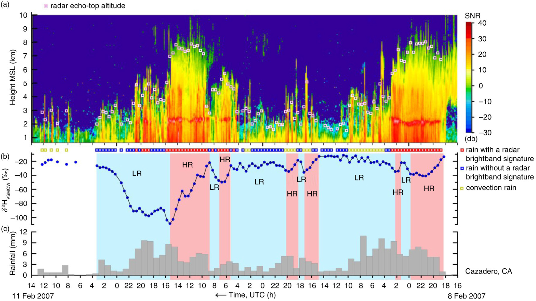
Fig. 5
(a) Time-height section of equivalent radar reflectivity factor with signal-to-noise ratio (SNR), (b) time series of δ 2HVSMOW values of 30-min, time-integrated precipitation samples and (c) histogram of hourly rainfall at Cazadero, CA, collected between 16 UTC 8 February 2007 and 14 UTC 11 February 2007. Open magenta squares indicate echo-top height. HR, pink panels, higher rainout, decreasing or low δ 2HVSMOW values. LR, blue panels, lower rainout, increasing or high δ 2HVSMOW values. Open red, blue, and yellow-gold squares indicate objective categorisation of rainfall occurring during selected half-hour periods. Time increases from right to left.
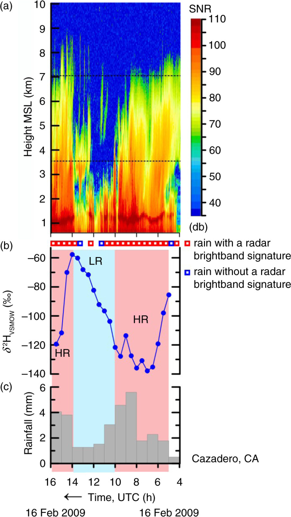
Fig. 6
(a) Time-height section of equivalent radar reflectivity factor with signal-to-noise ratio (SNR), (b) time series of δ 2HVSMOW values of 30-min, time-integrated precipitation samples, and (c) histogram of hourly rainfall at Cazadero, CA, collected between 4 and 16 UTC 16 February 2009. HR, pink panels, higher rainout, decreasing or low δ 2HVSMOW values. LR, blue panel, lower rainout, increasing or high δ 2HVSMOW values. Open squares indicate objective categorisation of the rainfall occurring during selected half-hour periods. Dashed horizontal lines are KMUX NEXRAD 0.5-degree beam. Time increases from right to left.
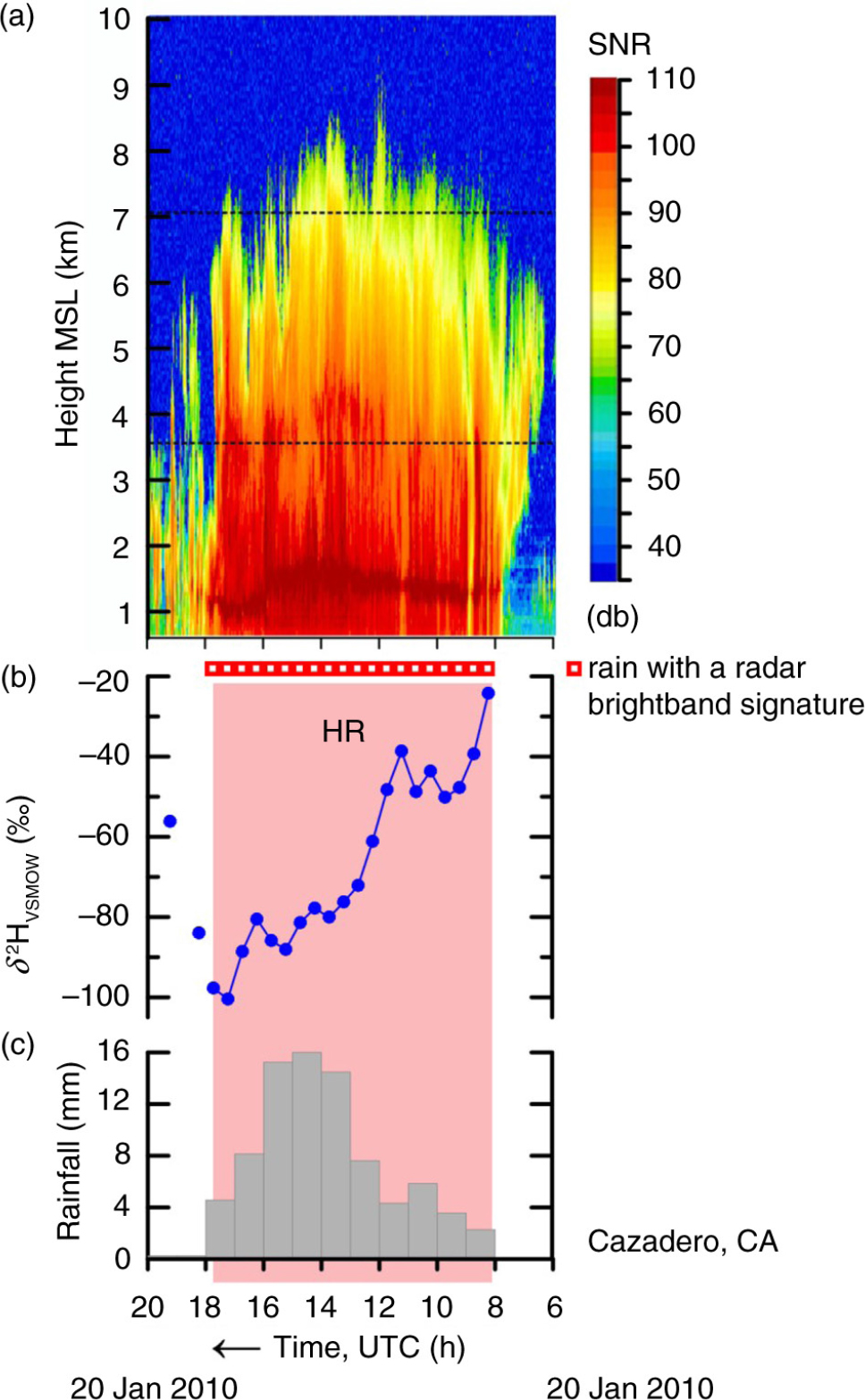
Fig. 7
(a) Time-height section of equivalent radar reflectivity factor with signal-to-noise ratio (SNR), (b) time series of δ 2HVSMOW values of 30-min, time-integrated precipitation samples and (c) histogram of hourly rainfall at Cazadero, CA, collected between 6 and 20 UTC 20 January 2010. HR, pink panel, higher rainout, decreasing or low δ 2HVSMOW values. Open squares indicate objective categorisation of the rainfall occurring during selected half-hour periods. Dashed horizontal lines are KMUX NEXRAD 0.5-degree beam. Time increases from right to left.
Applying algorithmic-isotopic categorisation of rainfall, we have created 82 pink panels in figures herein, including figures in the Section 7. Figures 7 and 9 show the wide variation in the duration of HR periods observed in this study. The duration of the HR period of the 19 January 2010 event at CZD (Fig. 9 and Table 2) is 3.5 h, whereas that of the 20 January 2010 event at CZD is 9.5 h (Fig. 7 and Table 2). Figure 7 shows a short-lived increase in δ 2HVSMOW of rainfall at 11 UTC. During this time, the BBY wind profiler time–height sections show uninterrupted warm-advection southerly component flow, and there is no indication of a significant meteorological transition aloft. The surface meteorological data at both BBY and CZD show no evidence of a meteorological transition at the surface. This is an example where application of rule 2 is appropriate. Although the duration of HR periods can be as great as 26 h, the average duration of HR periods is 3.6 h, with about 75 % of the HR periods having a duration of <6 h (Fig. 10a). Although δ 2HVSMOW decreases with time were as high as 44.3 ‰ h−1 (for BBY at 0730 UTC 22 February 2009), most values ranged between 4 and 16 ‰ h−1 (Fig. 11a).
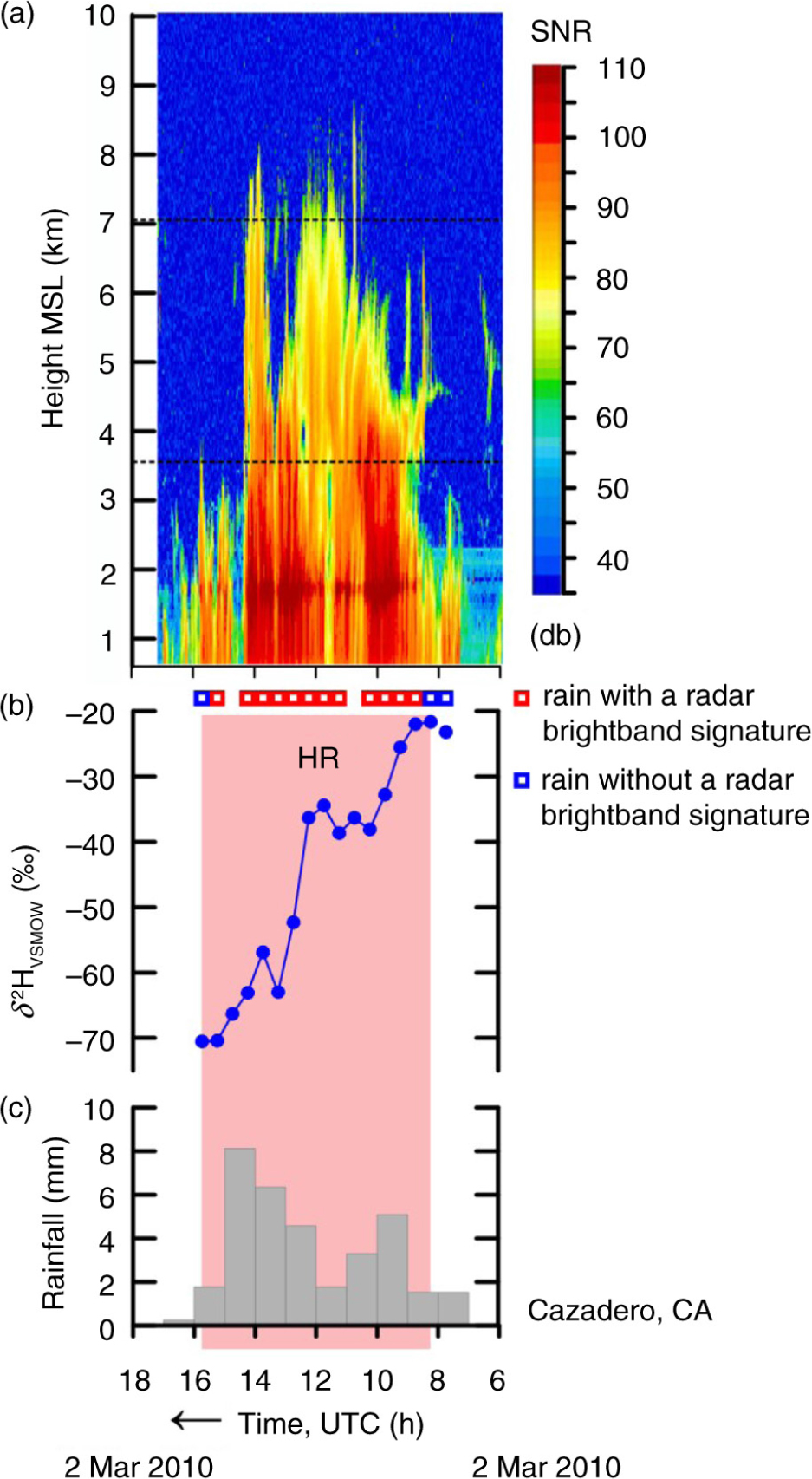
Fig. 8
(a) Time-height section of equivalent radar reflectivity factor with signal-to-noise ratio (SNR), (b) time series of δ 2HVSMOW values of 30-min, time-integrated precipitation samples and (c) histogram of hourly rainfall at Cazadero, CA, collected between 6 and 18 UTC 2 March 2010. HR, pink panel, higher rainout, decreasing or low δ 2HVSMOW values. Open squares indicate objective categorisation of the rainfall occurring during selected half-hour periods. Dashed horizontal lines are KMUX NEXRAD 0.5-degree beam. Time increases from right to left.
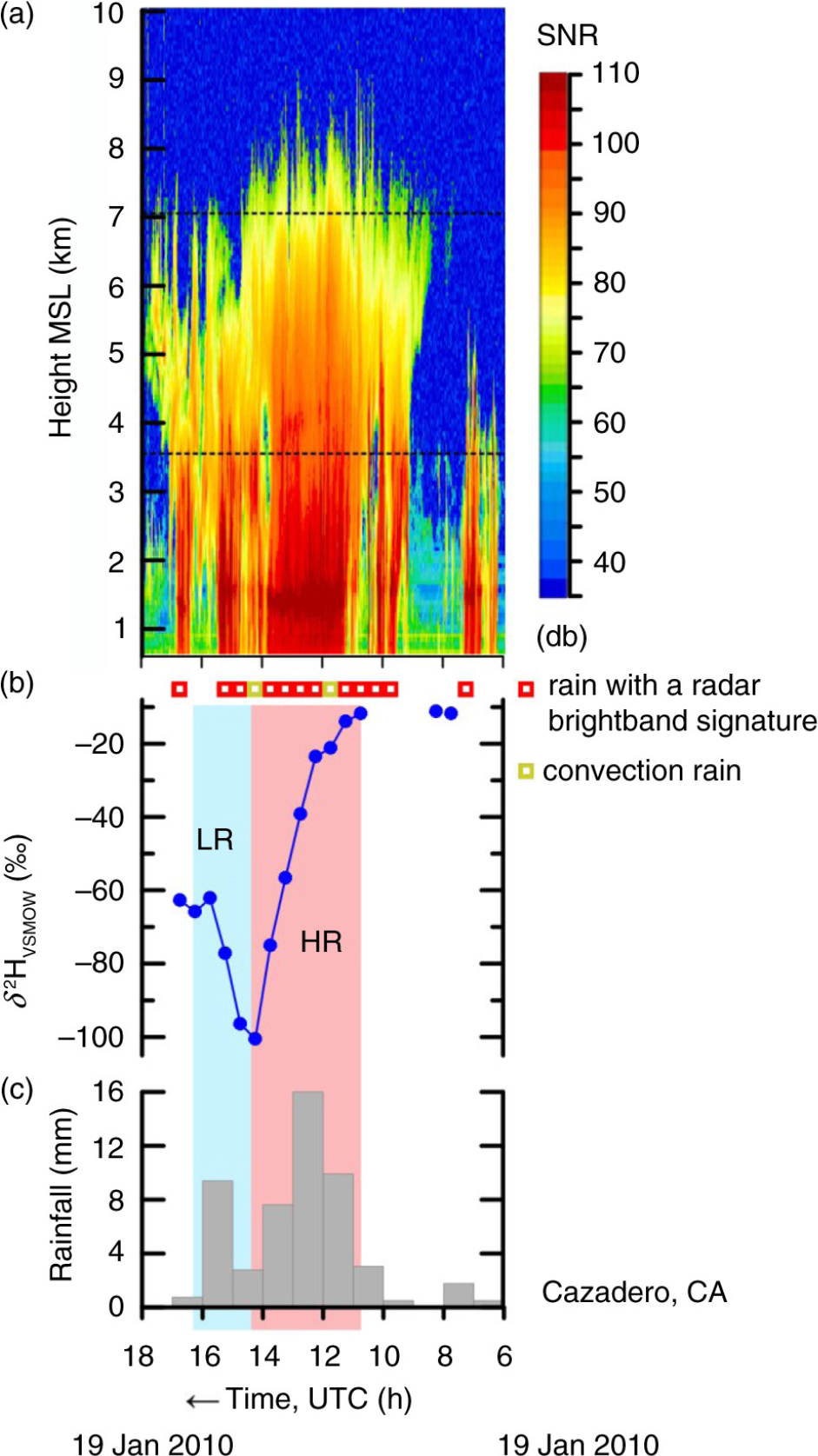
Fig. 9
(a) Time-height section of equivalent radar reflectivity factor with signal-to-noise ratio (SNR), (b) time series of δ 2HVSMOW values of 30-min, time-integrated precipitation samples and (c) histogram of hourly rainfall at Cazadero, CA, collected between 6 and 18 UTC 19 January 2010. HR, pink panel, higher rainout, decreasing or low δ 2HVSMOW values. LR, blue panel, lower rainout, increasing δ 2HVSMOW values. Open squares indicate objective categorisation of the rainfall occurring during selected half-hour periods. Dashed horizontal lines are KMUX NEXRAD 0.5-degree beam. Time increases from right to left.
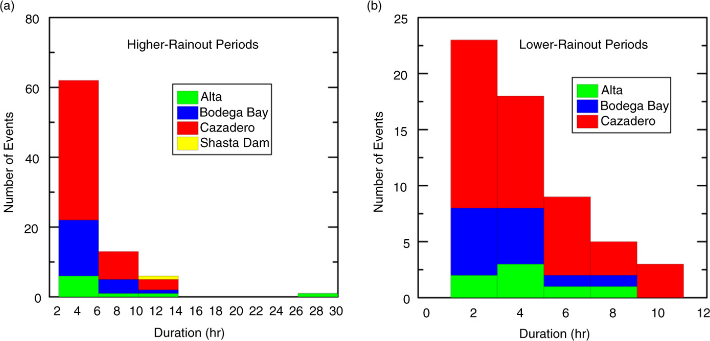
Fig. 10
Histograms of duration of rainout periods in this study. (a) Durations for higher rainout periods and (b) durations for lower rainout periods. Data are from Table 2.
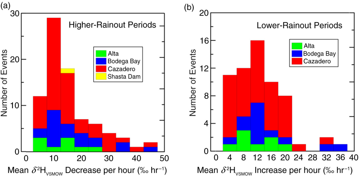
Fig. 11
Histograms of change in δ 2HVSMOW differences with time for sites in this study. (a) Peak-to-peak decreases in δ 2HVSMOW values with time for higher rainout periods and (b) peak-to-peak increases in δ 2HVSMOW values with time for lower rainout periods. Data are from Table 2.
Applying algorithmic-isotopic categorisation of rainfall, we have created 61 blue panels in figures herein, including figures in the Section 7.0. Although the duration of LR periods can be as great as 12.5 h, the duration of more than half of LR periods range between 1 and 5 h (Fig. 10b). Although δ 2HVSMOW increases with time were as high as 33.6 ‰ h−1 (for the BBY at 1715 UTC 18 January 2010), most values ranged between 6 and 18 ‰ h−1 (Fig. 11b).
Although about half of the 43 events in this study have a single HR period and (or) LR period, in many cases the increase in δ 2HVSMOW of precipitation of a LR period transitions back into a second HR period, with a substantial decrease in δ 2HVSMOW of precipitation. This is exemplified by Fig. 5 and by data from CZD from 16 February 2009 (Fig. 6); note that additional precipitation samples could not be collected after 1600 UTC 16 February 2009 because the sample carousel was full.
Occasionally, an event will consist solely or primarily of an HR period. An example is CZD between 0600 and 1800 UTC 2 March 2010 (Fig. 8), which had a decrease in δ 2HVSMOW of 48.9 ‰ over 7.5 h (Table 2). Other similar examples are shown in Fig. 7, Figs. A4, A25, A29, A33, A35 and A38. The CZD event shown in Fig. 8 shows a temporary weakening of BB precipitation between 10 and 12 UTC 2 March 2010. The BBY wind profiler time-height section shows uninterrupted warm-advection southerly component flow throughout this period; thus, there is no indication of a significant meteorological transition aloft and application of rules 2 and 3 is fully justified.
4.4. Correlations between δ2HVSMOW time series of neighbouring sites
When an air mass passes from one site to another during the landfall of an extratropical cyclone, there can be a strong correlation between the δ 2HVSMOW time series from the two sites. Most of the events in this study do not have a high correlation; however, three events do correlate well and are presented in this section. Recognising that BBY is a coastal site and that CZD is a nearby coastal mountain site that receives precipitation enhancement by orography, Fig. 12 compares BBY and CZD on 22 February 2009. The distance between BBY and CZD is 35 km. The collection time of each CZD sample has been decreased by 9 min to account for travel time of the air mass from BBY to CZD. This time offset gives the highest cross-correlation value of the two time series (0.65). The transit time seems too fast to us, but this is the value determined by calculating the δ 2HVSMOW value of each time series minute by minute using linear extrapolation between 30-min data points and then calculating the offset time for maximum cross correlation. One problem in estimating transit time is that we do not know the precise direction(s) responsible for the advection of precipitation, given that the precipitation is likely originating from different directions at different levels.
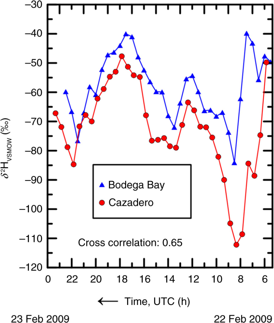
Fig. 12
Comparison of δ 2HVSMOW of Bodega Bay and Cazadero, CA, precipitation between 6 UTC 22 February 2009 and 0 UTC 23 February 2009. Time increases from right to left. The time of each CZD sample has been decreased by 9 min to account for travel time of the air mass from Bodega Bay to Cazadero.
Figure 13 compares BBY and CZD between 2000 UTC 17 January 2010 and 2000 UTC 18 January 2010. The collection time of each CZD sample has been decreased by 32 min to account for travel time of the air mass from BBY to CZD. This time offset gives the highest cross-correlation value of the two δ 2HVSMOW time series (0.989). The average south to southwest flow at BBY during this event was probably in the order of 15-30 m s−1; thus, we would expect a faster transit time than 32 min, and we cannot explain this longer transit time, but it is likely related to the fact that, as above, we do not know the precise direction(s) responsible for the advection of precipitation, given that the precipitation is likely originating from different directions at different levels.
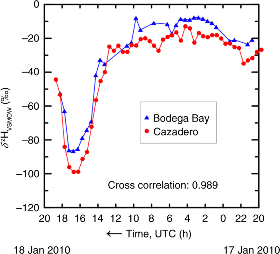
Fig. 13
Comparison of δ 2HVSMOW of Bodega Bay and Cazadero,CA, precipitation between 20 UTC 17 January 2010 and 20 UTC 18 January 2010. Time increases from right to left. The collection time of each CZD sample has been decreased by 32 min to account for travel time of the air mass from Bodega Bay to Cazadero.
The δ 2HVSMOW profile of BBY is, on average, more positive than that of CZD in both examples because the elevation of CZD (475 m) is higher (i.e. colder) than that of BBY (12 m). The mean differences between the two δ 2HVSMOW time series in Fig. 12 and 13 are 14.8 and 8.6 ‰, respectively. This phenomenon is termed the altitude effect. Assuming an average difference of 11.6 ‰, the altitude effect is calculated as −11.6 ‰/463 m=−2.5 ‰ per 100 m in which we assume the difference in condensation heights over CZD and BBY is the same as the difference in terrain height (463 m). For a thorough evaluation of the altitude effect, one should consider the lifted condensation level (LCL) relative to the altitude at both sites. Because CZD would likely have a higher relative humidity than that of BBY, the difference in the LCL between BBY and CZD would likely be somewhat <463 m. But this detailed evaluation of the LCL is beyond the scope of this work. This value of −2.5 ‰ per 100 m compares satisfactorily with −4 ‰ per 100 m in France reported by Moser and Stichler (1970), −2.5 ‰ per 100 m in Italy reported by Bortolami et al. (1979), and −1 ‰ per 100 m in Nevada reported by Friedman et al. (2002). The equivalent altitude effect for the oxygen-isotope data is −0.3 ‰ per 100 m. Such variations in isotopic composition with elevation are important for aiding hydrologists in identifying the source(s) of groundwater.
Figure 14 compares CZD and ATA between 1600 UTC 23 February 2008 and 0800 UTC 24 February 2008. The collection time of each ATA sample has been decreased by 200 min to account for travel time of the air mass from CZD to ATA, which are 210 km apart. This time offset gives a cross-correlation value of 0.60. During this interval, the wind profiler at BBY indicated a strong southerly component flow on the order of 20 m s−1 and the south-to-north distance between these sites is ~69 km. Thus, the apparent time difference of 200 min is too great, and we are unable to explain this higher travel time. Over this period, the average difference in δ 2HVSMOW is 11.1 ‰. The elevation of ATA is 1085 m (Table 1); thus, the altitude effect is −11.1 ‰/(1085 m – 475 m)=−1.8 ‰ per 100 m, identical to than that determined between BBY and CZD above. The equivalent altitude effect for the oxygen-isotope data is −0.2 ‰ per 100 m. The above correlations between the δ 2HVSMOW time series at two sites provide input data to test regional-scale and global-scale isotope-enabled climate models (Buenning et al., 2012).
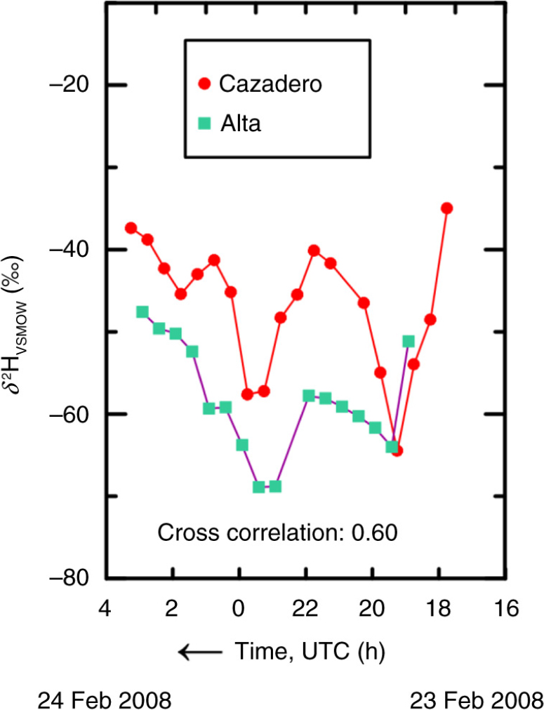
Fig. 14
Comparison of δ 2HVSMOW of Cazadero and Alta, CA, precipitation between 16 UTC 23 February 2008 and 8 UTC 24 February 2008. Time increases from right to left. The collection time of each Alta sample has been decreased by 200 min to account for travel time of the air mass from Cazadero to Alta.
4.5. Rainfall rate, accumulated rainfall and hydrogen isotopic composition
To investigate the correlations during HR and LR periods between accumulated rainfall and the peak-to-peak δ 2HVSMOW differences of precipitation during these events, accumulated rainfall (Table 2) is plotted against δ 2HVSMOW difference (Table 2) in Fig. 15. The R 2 values for ATA, BBY and CZD for HR periods (Fig. 15a) are 0.90, 0.24 and 0.22, respectively. The R 2 values for ATA, BBY and CZD for LR periods (Fig. 15b) are 0.24, 0.11 and 0.20, respectively. The correlations for BBY and CZD are weak. Although the correlation for HR periods from ATA is high, this is due primarily to a single point in Table 2 (δ 2HVSMOW difference=91.4 ‰ and accumulated rainfall=64.52 mm) out of only nine values at ATA. Thus, it is concluded that there is little to no correlation between the magnitude of HR periods or LR periods and accumulated rainfall. Therefore, δ 2HVSMOW decreases/increases cannot be used as predictors of rainfall magnitude.
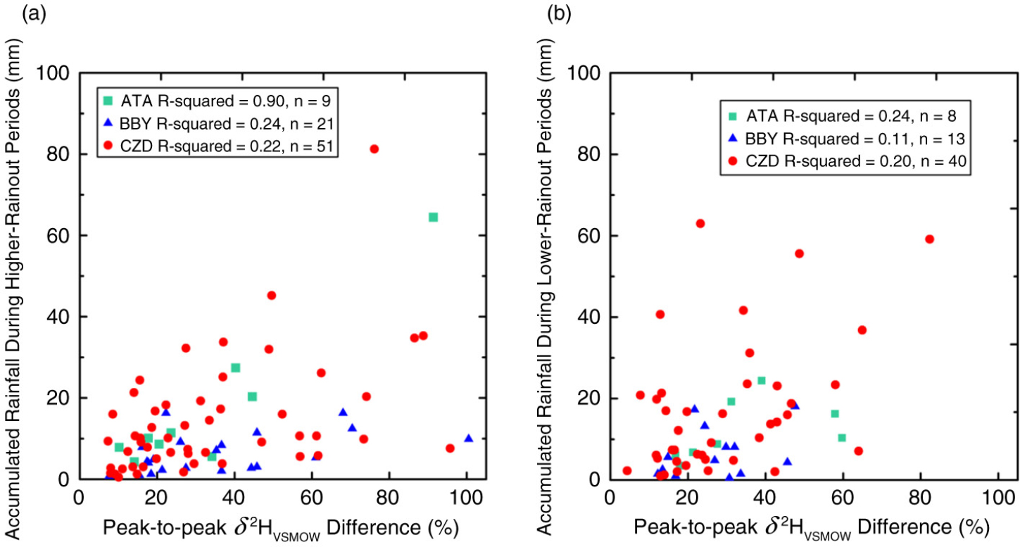
Fig. 15
Comparison of accumulated rainfall at Alta (ATA), Bodega Bay (BBY) and Cazadero (CZD) with peak-to-peak δ 2HVSMOW differences. (a) During higher rainout periods and (b) during lower rainout periods. Data are from Table 2.
To investigate the correlations during HR and LR periods between mean rainfall rate and changes in δ 2HVSMOW values of precipitation, mean rainfall rates were calculated from data in Table 2 and plotted against peak-to-peak δ 2HVSMOW differences (Table 2); they are shown in Fig. 16. The R 2 values for ATA, BBY and CZD for HR periods (Fig. 16a) are 0.09, 0.06 and 0.04, respectively. The R 2 values for ATA, BBY and CZD for LR periods (Fig. 16b) are 0.18, 0.00 and 0.06, respectively. The correlations between mean rainfall rate and peak-to-peak δ 2HVSMOW differences are nearly non-existent. Hence, as was the case for accumulated rainfall, δ 2HVSMOW decreases and increases cannot be used as predictors of the rainfall intensity.
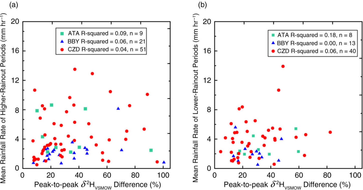
Fig. 16
Comparison of mean rainfall rate at Alta (ATA), Bodega Bay (BBY) and Cazadero (CZD) with peak-to-peak δ 2HVSMOW differences. (a) During higher rainout periods and (b) during lower rainout periods. Data are from Table 2.
To investigate the correlation between accumulated rainfall during an event and minimum δ 2HVSMOW of precipitation during that event, accumulated-event rainfall was calculated from data in Table 2. Figure 17 presents a plot of accumulated-event rainfall versus minimum δ 2HVSMOW of precipitation for each CZD and ATA event (31 events total). The correlation between accumulated-event rainfall and minimum-event δ 2HVSMOW of precipitation is meaningful, but low (R 2=0.19). Fifteen of the events in Fig. 17 have been classified as ARs. Of the 31 events in which isotopic measurements were obtained at CZD and ATA (Fig. 17), 15 have been classified as ARs (Neiman et al., 2008; Dettinger et al., 2011; Ralph et al., 2013b). We found that average minimum δ 2HVSMOW valuesof AR rainfall at CZD and ATA (−92.8 ‰, n=15) were substantially lower than the average minimum δ 2HVSMOW value of non-AR events (−65.2 ‰, n=16). Of the five events having the lowest δ 2HVSMOW values (precipitation from deep, cold cloud layer), all occurred with California ARs (Fig. 17). The remarkable AR of 16 February 2009 (Fig. 17) had the lowest δ 2HVSMOW value of rainfall at CZD in our study (−137.9 ‰), which is ~55 ‰ lower than that of the 21–22 March 2005 event at CZD investigated by Coplen et al. (2008), in accord with involvement of colder, deeper clouds (> 6.5 km altitude). In Fig. 17, all events with δ 2HVSMOW values of rainfall at CZD below −105 ‰ were ARs. Of the 13 events having δ 2HVSMOW values of rainfall below −80 ‰, 77 % (10) are ARs. Many of the ARs do not have low δ 2HVSMOW values of precipitation, and we surmise that the most intense part of these ARs did not intercept CZD or ATA, but rather were either centred north or south of these sites.
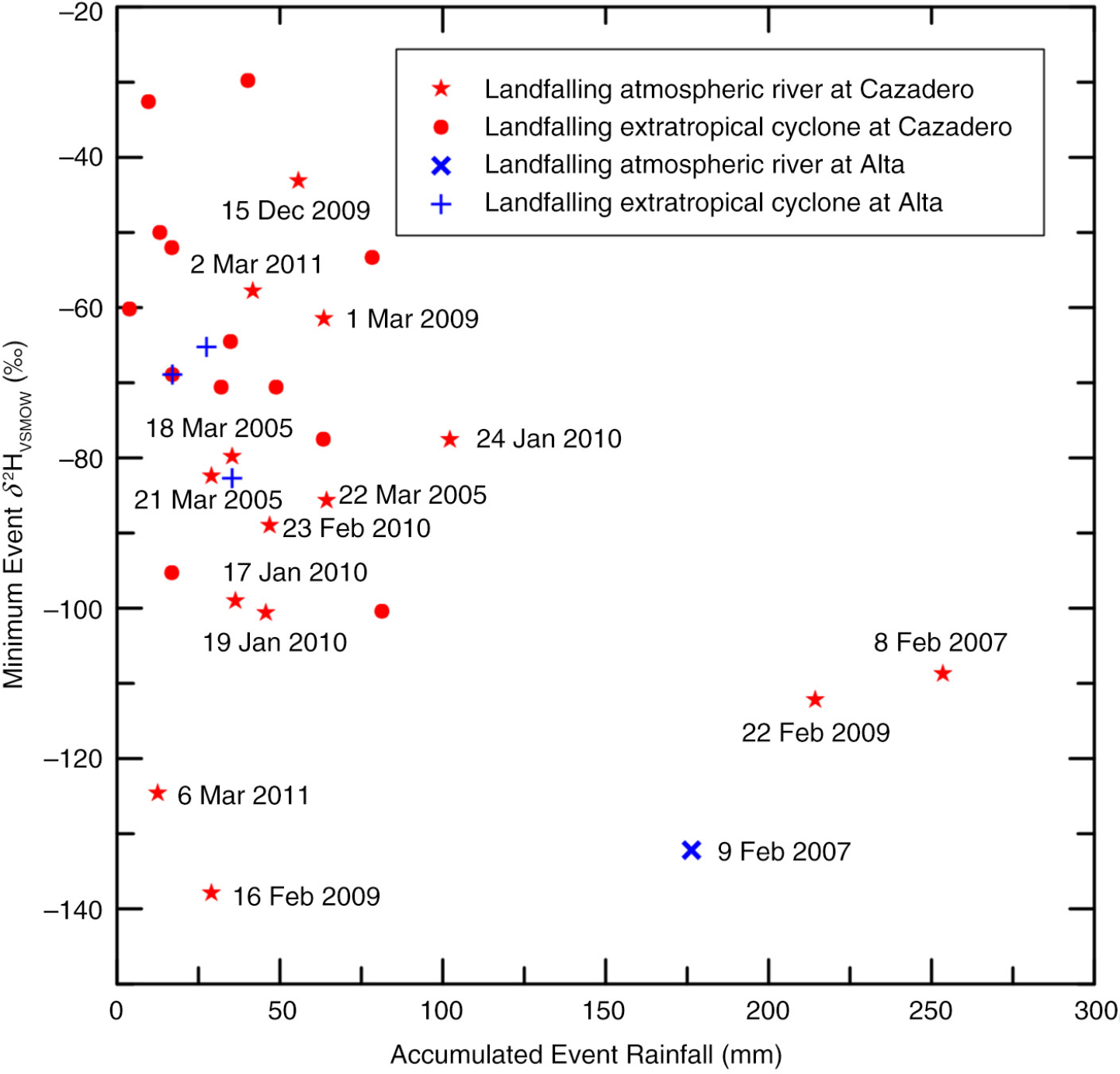
Fig. 17
Accumulated-event rainfall versus minimum δ 2HVSMOW values of rainfall of 27 CZD and 4 ATA events in this study. Landfalling atmospheric rivers are long, narrow plumes of integrated water vapour with core values >~2 cm that impacted the California coast (Neiman et al., 2008; Dettinger et al., 2011; Ralph et al., 2013a).
4.6. Relation between radar echo-top heights and hydrogen isotopic composition
Scholl et al. (2009) observed that seasonal difference in NEXRAD cloud echo-top heights and their corresponding temperatures were correlated with the isotopic composition of rainfall in Puerto Rico. Echo-top heights derived from S-PROF radar reflectivity profiles are available for selected CZD and ATA events and are provided in the Supplementary File. Previous work (Martner et al., 2008) indicated that the mean echo-top height was higher (6.8 km, corresponding to −26.3 °C) for BB periods and lower (3.6 km, corresponding to −5.6 °C) for NBB periods, in accord with HR periods being colder with lower δ 2HVSMOWvalues of precipitation and LR periods being warmer with higher lower δ 2HVSMOW values of precipitation. Figure 5 shows echo-top heights for CZD between 1845 UTC 8 February 2007 and 1215 UTC 11 February 2007. HR-period echo-top heights are greater on average than those of LR periods, and the average BB height (height of maximum radar reflectivity) represents the freezing level and was 2.31 km above mean sea level. In this study, 2 ATA and 21 CZD events have at least one HR period, one LR period and echo-top heights. We have calculated the mean-event echo-top height for HR and LR periods. In Fig. 18, we plot the minimum-event δ 2HVSMOW value of precipitation versus the mean-event HR-period echo-top height. Similarly, we plot the maximum-event δ 2HVSMOW value of precipitation versus the mean-event LR-period echo-top height. Echo-top heights are strongly correlated with δ 2HVSMOW values of precipitation because they are a proxy for temperature. For 22 of the 23 plots in Fig. 18, the mean echo-top height is greater for HR periods than that for LR periods, in accord with isotope–hydrology expectations. However, for one unusual event (17 January 2010 at CZD), shown in Fig. A15, the reverse situation is observed because the interval between 1715 and 1845 UTC with strongly increasing δ 2HVSMOW values of precipitation has been classified as a LR period, apparently incorrectly. The reason for the unexpected 45.6 ‰ increase in δ 2HVSMOW of precipitation during this 1.5-h interval is unknown. Using cloud echo-top altitudes combined with isotopic compositions enables researchers to trace groundwater recharge to climate patterns and inform studies of climate change.
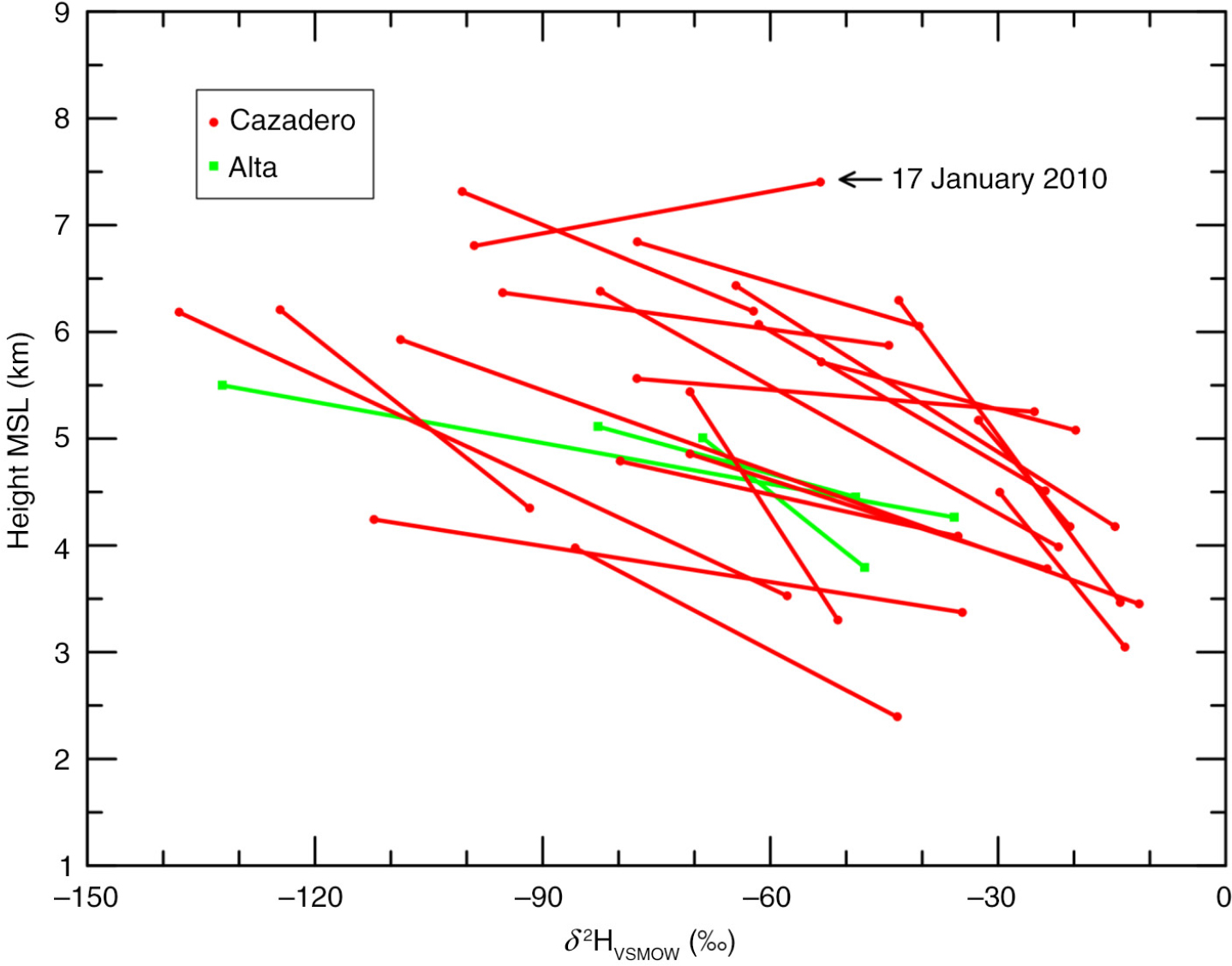
Fig. 18
Mean echo-top height of HR and LR periods versus maximum δ 2HVSMOW of rainfall for each LR period and minimum δ 2HVSMOW values of rainfall for each HR period for 21 Cazadero and 2 Alta events having echo-top data. The mean echo-top height of the HR period of the Cazadero 17 January 2010 event (Fig. A15) is lower than that of its LR period.
4.7. Potential for improving hydrograph separation
The separation of storm hydrographs using stable-isotope tracers dates back to the late 1960s (Hubert et al., 1969; Dinçer et al., 1970). These studies ushered in a paradigm shift in how hydrologists conceptualised runoff generation as most showed a large fraction of pre-event water in the storm hydrograph, even at peak flow (Turner and Barnes, 1998; Klaus and McDonnell, 2013). Theories that invoked rainfall translation to streamflow as overland flow and rainfall translation to streams by lateral, preferential flow required substantial revision once hydrograph separations using environmental hydrogen and oxygen isotopes showed that stored, pre-event water dominated the storm hydrograph in most humid systems (Sklash et al., 1976). This forced a fundamental re-examination of the processes of water delivery to streams during rainfall and snowmelt events (Klaus and McDonnell, 2013). Despite several limitations, stable hydrogen and oxygen-isotope measurements continue to be the best conservative tracer for water among those currently available because they are part of the water molecule. Once free from evaporative exposure, they are only subject to changes due to mixing (Kendall and McDonnell, 1998). Typically, environmental stable hydrogen and oxygen-isotope measurements are used in catchment hydrology studies to (1) determine the mechanisms and processes involved in the generation and discharge of streamflow, (2) estimate residence-time distributions of water within the catchment, (3) determine the origin of streamflow components, (4) calibrate or validate catchment streamflow models, (5) predict catchment response and (6) estimate hydrologic parameters (Turner and Barnes, 1998).
Hydrograph separation is based on the following five assumptions (Sklash et al., 1976; Sklash and Farvolden, 1979; Moore, 1989; Buttle, 1994; Klaus and McDonnell, 2013):
The isotopic content of the event and the pre-event water are significantly different.
The event water maintains a constant isotopic signature in space and time, or any variations can be accounted for.
The isotopic signature of the pre-event water is constant in space and time, or any variations can be accounted for.
Contributions from the vadose zone must be negligible, or the isotopic signature of the soil water must be similar to that of groundwater.
Surface storage contributes minimally to the streamflow.
Quantification of the isotopic composition of event precipitation to evaluate assumption 2 has been performed by collection of precipitation samples at 2-h to 1-month intervals (Klaus and McDonnell, 2013). Herein, we observed variations in δ 2HVSMOW of rainfall of as much as ~100 ‰ over a few hours. By using an input method that accounts for time variance in the isotopic composition of precipitation, such as TRANSEP (Weiler et al., 2003), improved determination of storm hydrograph parameters, especially on hourly time periods, ought to be possible.
4.8. Comparison of algorithmic-isotopic categorisation of precipitation with objective categorisation of precipitation by S-Prof radar
Figure 18 shows the strong correlation between mean echo-top heights of HR and LR periods and minimum δ 2HVSMOW of values of rainfall for 23 events having echo-top data. Because BB rainfall has higher mean echo-top heights than NBB rainfall (Martner et al., 2008), we anticipate that there may be a correlation between intervals having precipitation categorised by S-Prof radar as BB rain and intervals categorised as HR periods using algorithmic-isotopic categorisation of precipitation. Similarly, we anticipate that there may be a correlation between intervals having precipitation objectively categorised as NBB rain and periods categorised as LH periods.
There are 25 CZD events and 1 ATA event having precipitation categorised by S-Prof radar. In Table 3, we have tabulated for each event (1) the number of BB squares having a rainfall rate >0.6 mm h−1 for a minimum of 1 h, (2) the number of BB squares associated with an HR period, (3) the number of NBB squares having a rainfall rate >0.6 mm h−1 for a minimum of 1 h and (4) the number of NBB squares associated with a LR period. The rainfall rate of 0.6 mm h−1 is specified because this minimum rainfall rate is specified in the rules (criteria) for algorithmic-isotopic categorisation of precipitation. There are 420 BB-categorised squares with these criteria in these 26 events, and 278 occur during HR periods. Thus, the algorithmic-isotopic categorisation of precipitation captures about two-thirds of the BB rain. There are 252 BB-categorised squares with these criteria in these events, and 150 occur during LR periods. Thus, the algorithmic-isotopic categorisation of precipitation captures about three-fifths of the NBB rain. Thus, a conclusion of this study is that algorithmic-isotopic categorisation of rainfall is potentially useful for identifying periods of BB and NBB rain. As an example, radar reflectivity instrumentation was not operational at CZD during the event 23–24 February 2010 (Fig. A18). Between 2145 and 2345 UTC 23 February 2010, δ 2HVSMOW of rainfall decreased by 73.4 ‰ (Table 2), and the rain collected during this interval would be classified as BB rain based on the δ 2HVSMOW measurements. Between 2345 UTC 23 February 2010 and 0815 UTC 24 February 2010, δ 2HVSMOW of rain increased by 64.9 ‰ (Table 2), and the rain collected during this interval would be classified as NBB rain based on δ 2HVSMOW measurements.
Table 3. Count of objective categorisation of rainfall for events having radar brightband signature data at 30-min intervals
4.9. Evaluation of kinetic isotopic exchange between falling droplets and ambient water vapour below the cloud base
Friedman et al. (1962) were among the first to demonstrate in an environmental setting that rain falling through a dry air column will evaporate and become enriched in the heavy isotopes of water (2H and 18O). This phenomenon is the primary cause of the ‘amount effect’ in an event (Dansgaard, 1964). This kinetic isotopic fractionation is best observed in arid regions, such as Bahrain in the Arabian Gulf, and it is accompanied by a slope in a plot of δ 2HVSMOW versus δ 18OVSMOW of precipitation of substantially <8 (Clark and Fritz, 1997) because 18O is enriched preferentially over 2H in falling raindrops. Once the air column becomes saturated, there is no potential for kinetic isotopic fractionation, and the slope increases to the equilibrium value of 8 (Clark and Fritz, 1997). Yoshimura et al. (2010) used the isotope-abundance measurements of the March 2005 storm event (Coplen et al., 2008) in a regional model for simulations of the March 2005 storm. They conducted a set of sensitivity experiments and comparisons with observations and concluded that the kinetic isotopic exchange between falling droplets and ambient water vapour below the cloud base, as observed by Friedman et al. (1962), was mostly responsible for the initial enrichment and subsequent rapid drop of the δ 2HVSMOW value of precipitation observed during the event, even under humid conditions. Their hypothesis relies on non-equilibrium (kinetic) isotopic exchange or fractionation of water in droplets falling from a cloud and vapour below the cloud. If the hypothesis of Yoshimura et al. (2010) were correct, one ought to find a slope <8 in a δ 2HVSMOW−δ 18OVSMOW relationship. Figure 19 presents a δ 2HVSMOW versus δ 18OVSMOW crossplot of precipitation from the 21–22 March 2005 event studied by Coplen et al. (2008). The slope of the isotopic data in the Periods II and III in Fig. 2 of Coplen et al. (2008) is 8.12, shown as a pink line in Fig. 19, and it is in excellent agreement with the slope of the global meteoric water line of Rozanski et al. (1993) of 8.2, given in eq. (2). We conclude that the proposed processes and conclusions of Yoshimura et al. (2010) are unsupportable because (1) water vapour below clouds of a storm would quickly reach isotopic equilibrium with falling water drops because the mass of water in rain drops is substantially greater than the mass of water in vapour in the column, (2) once the column becomes saturated, kinetic isotopic fractionation terminates and (3) the δ 2HVSMOW versus δ 18OVSMOW slope of rain drops undergoing kinetic isotopic fractionation should be substantially <8, but a slope of 8.12 was observed.
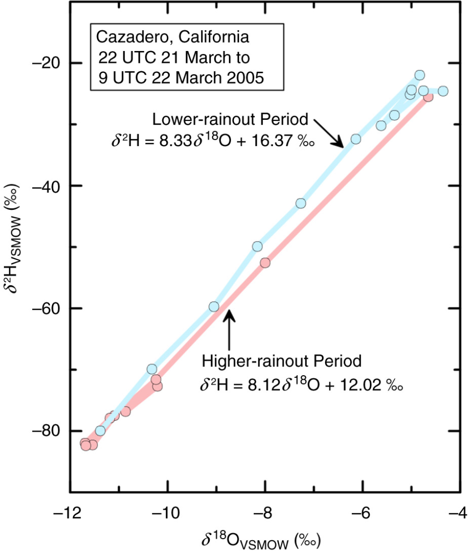
Fig. 19
Crossplot of δ 2HVSMOW and δ 18OVSMOW of precipitation collected on 21–22 March 2005 at Cazadero, CA.
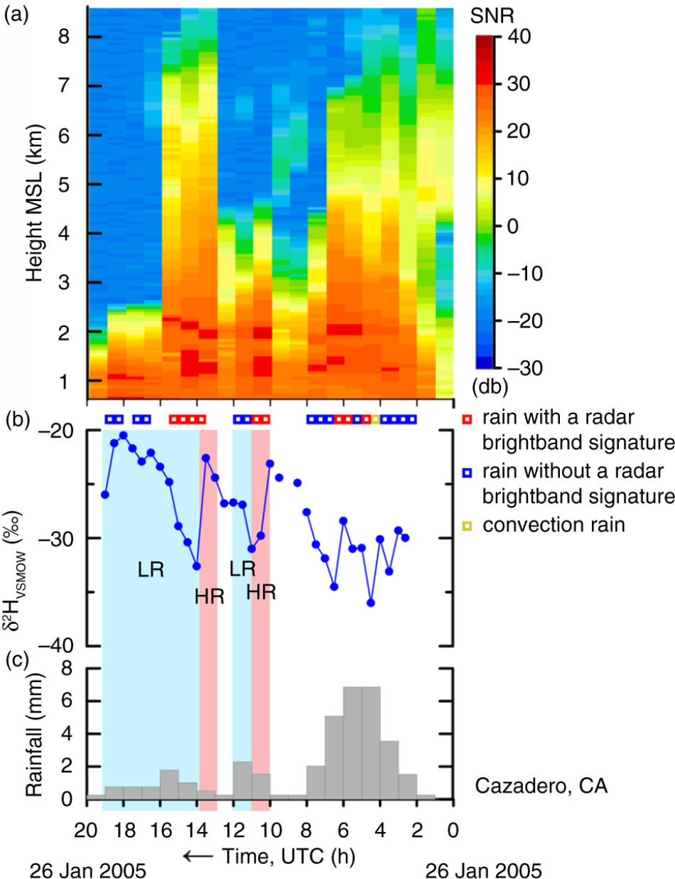
Fig. A1
(a) Time–height section of equivalent radar reflectivity factor with signal-to-noise ratio (SNR), (b) time series of δ 2HVSMOW values of 30-min, time-integrated precipitation samples and (c) histogram of hourly rainfall at Cazadero, CA, collected between 0 and 20 UTC 26 January 2005. HR, pink panels, higher rainout, decreasing or low δ 2HVSMOW values. LR, blue panels, lower rainout, increasing or high δ 2HVSMOW values. Open squares indicate objective categorization of the rainfall occurring during selected half-hour periods. Time increases from right to left.
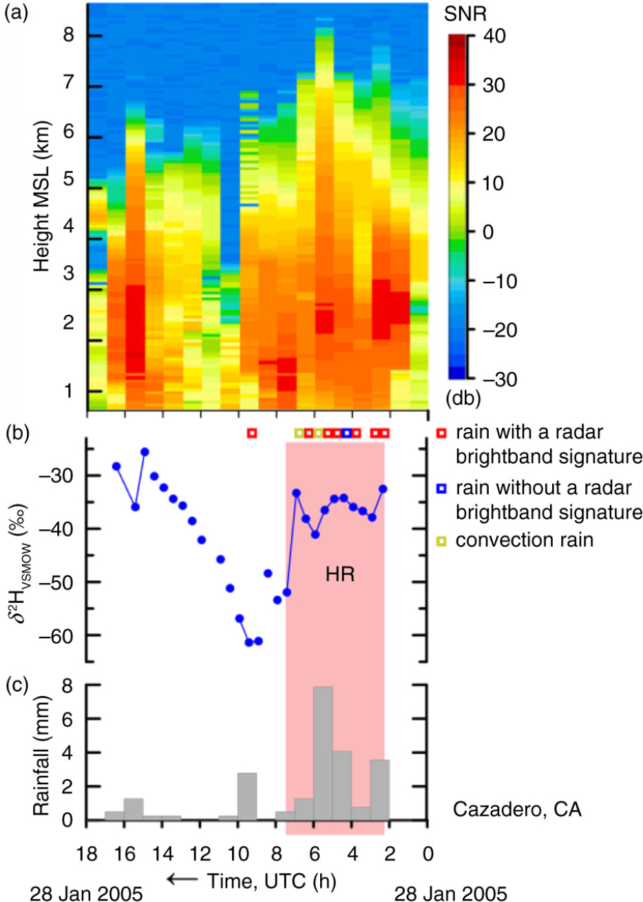
Fig. A2
(a) Time–height section of equivalent radar reflectivity factor with signal-to-noise ratio (SNR), (b) time series of δ 2HVSMOW values of 30-min, time-integrated precipitation samples and (c) histogram of hourly rainfall at Cazadero, CA, collected between 0 and 18 UTC 28 January 2005. Period A, pink panel, zone of decreasing or low δ 2HVSMOW values. HR, pink panel, higher rainout, decreasing or low δ 2HVSMOW values. Open squares indicate objective categorization of the rainfall occurring during selected half-hour periods. Time increases from right to left.
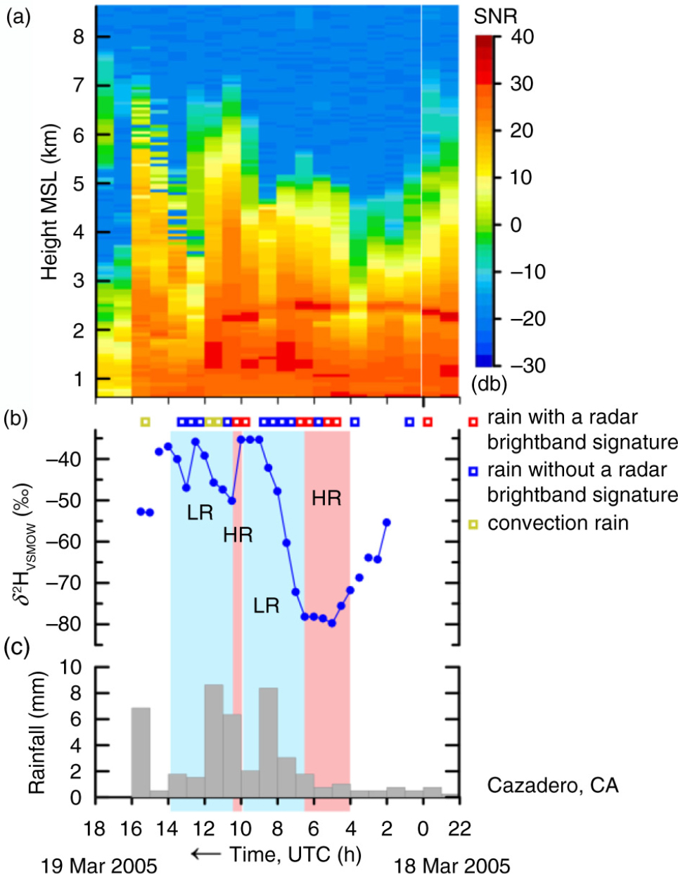
Fig. A3
(a) Time–height section of equivalent radar reflectivity factor with signal-to-noise ratio (SNR), (b) time series of δ 2HVSMOW values of 30-min, time-integrated precipitation samples and (c) histogram of hourly rainfall at Cazadero, CA, collected between 22 UTC 18 March 2005 and 18 UTC 19 March 2005. Period A, pink panel, zone of decreasing or low δ 2HVSMOW values. HR, pink panels, higher rainout, decreasing or low δ 2HVSMOW values. LR, blue panels, lower rainout, increasing or high δ 2HVSMOW values. Open squares indicate objective categorization of the rainfall occurring during selected half-hour periods. Time increases from right to left.
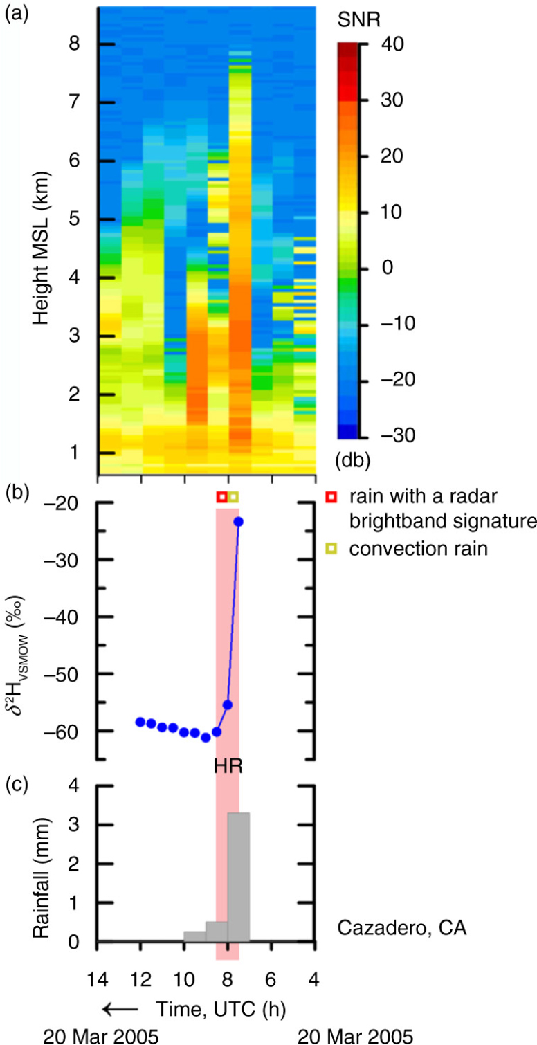
Fig. A4
(a) Time–height section of equivalent radar reflectivity factor with signal-to-noise ratio (SNR), (b) time series of δ 2HVSMOW values of 30-min, time-integrated precipitation samples and (c) histogram of hourly rainfall at Cazadero, CA, collected between 4 and 14 UTC 20 March 2005. HR, pink panel, higher rainout, decreasing or low δ 2HVSMOW values. Open squares indicate objective categorization of the rainfall occurring during selected half-hour periods. Time increases from right to left.
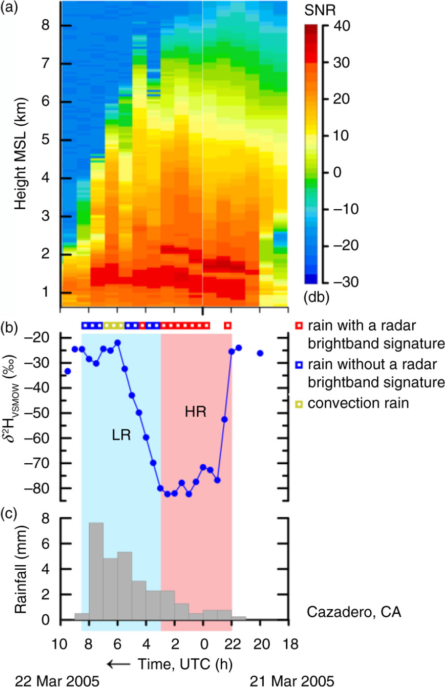
Fig. A5
(a) Time–height section of equivalent radar reflectivity factor with signal-to-noise ratio (SNR), (b) time series of δ 2HVSMOW values of 30-min, time-integrated precipitation samples and (c) histogram of hourly rainfall at Cazadero, CA, collected between 18 UTC 21 March 2005 and 10 UTC 22 March 2005. HR, pink panel, higher rainout, decreasing or low δ 2HVSMOW values. LR, blue panel, lower rainout, increasing or high δ 2HVSMOW values. Open squares indicate objective categorization of the rainfall occurring during selected half-hour periods. Time increases from right to left.
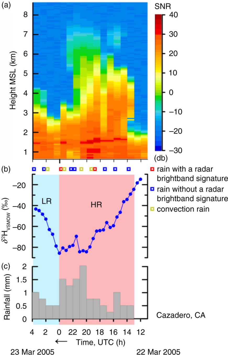
Fig. A6
(a) Time–height section of equivalent radar reflectivity factor with signal-to-noise ratio (SNR), (b) time series of δ 2HVSMOW values of 30-min, time-integrated precipitation samples and (c) histogram of hourly rainfall at Cazadero, CA, collected between 12 UTC 22 March 2005 and 4 UTC 23 March 2005. HR, pink panel, higher rainout, decreasing or low δ 2HVSMOW values. LR, blue panel, lower rainout, increasing or high δ 2HVSMOW values. Open squares indicate objective categorization of the rainfall occurring during selected half-hour periods. Time increases from right to left.
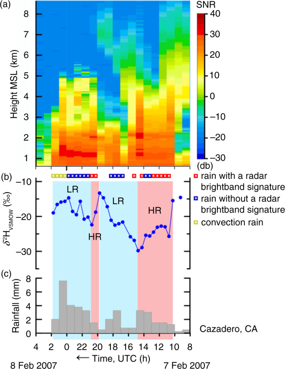
Fig. A7
(a) Time–height section of equivalent radar reflectivity factor with signal-to-noise ratio (SNR), (b) time series of δ 2HVSMOW values of 30-min, time-integrated precipitation samples and (c) histogram of hourly rainfall at Cazadero, CA, collected between 8 UTC 7 February 2007 and 4 UTC 8 February 2007. HR, pink panels, higher rainout, decreasing or low δ 2HVSMOW values. LR, blue panels, lower rainout, increasing or high δ 2HVSMOW values. Open squares indicate objective categorization of the rainfall occurring during selected half-hour periods. Time increases from right to left.
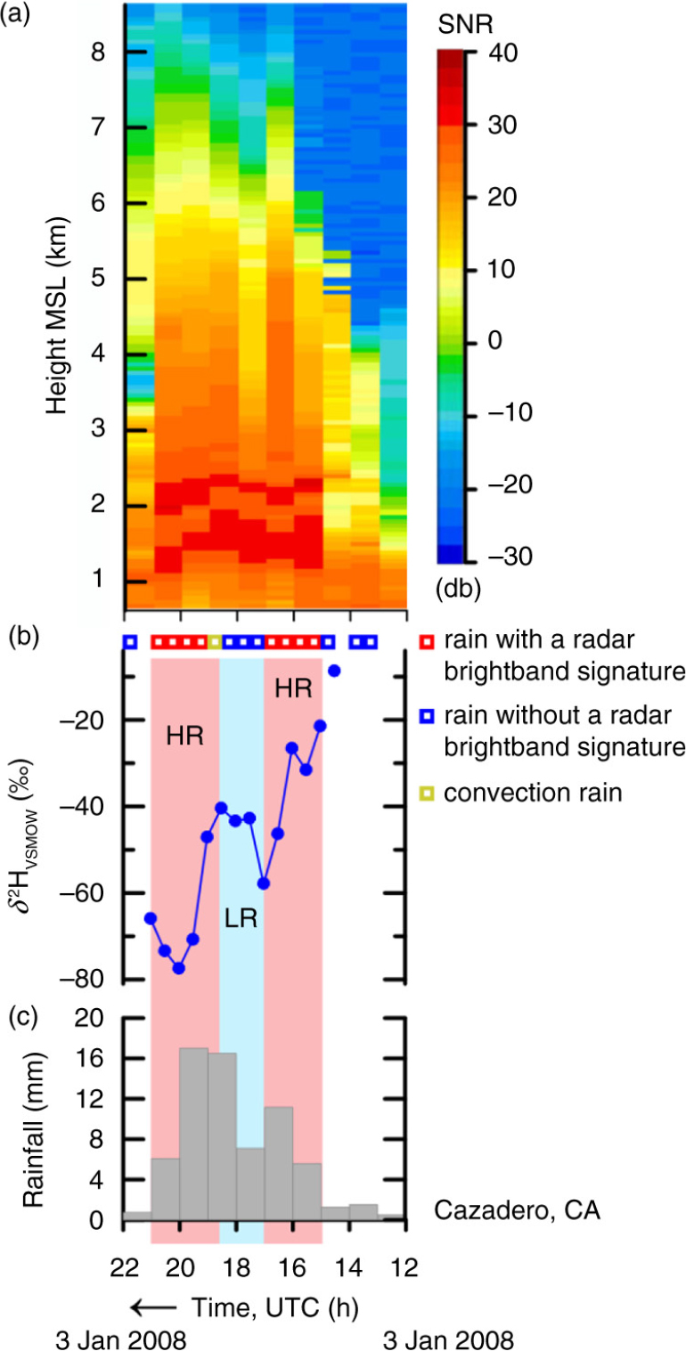
Fig. A8
(a) Time–height section of equivalent radar reflectivity factor with signal-to-noise ratio (SNR), (b) time series of δ 2HVSMOW values of 30-min, time-integrated precipitation samples and (c) histogram of hourly rainfall at Cazadero, CA, collected between 12 and 22 UTC 3 January 2008. HR, pink panels, higher rainout, decreasing or low δ 2HVSMOW values. LR, blue panel, lower rainout, increasing or high δ 2HVSMOW values. Open squares indicate objective categorization of the rainfall occurring during selected half-hour periods. Time increases from right to left.
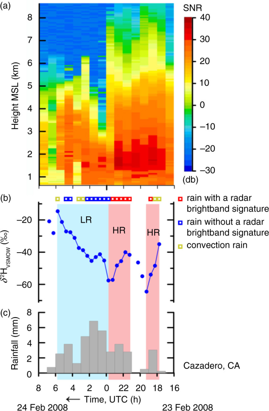
Fig. A9
(a) Time–height section of equivalent radar reflectivity factor with signal-to-noise ratio (SNR), (b) time series of δ 2HVSMOW values of 30-min, time-integrated precipitation samples and (c) histogram of hourly rainfall at Cazadero, CA, collected between 16 UTC 23 February and 8 UTC 24 February 2008. HR, pink panels, higher rainout, decreasing or low δ 2HVSMOW values. LR, blue panel, lower rainout, increasing or high δ 2HVSMOW values. Open squares indicate objective categorization of the rainfall occurring during selected half-hour periods. Time increases from right to left.
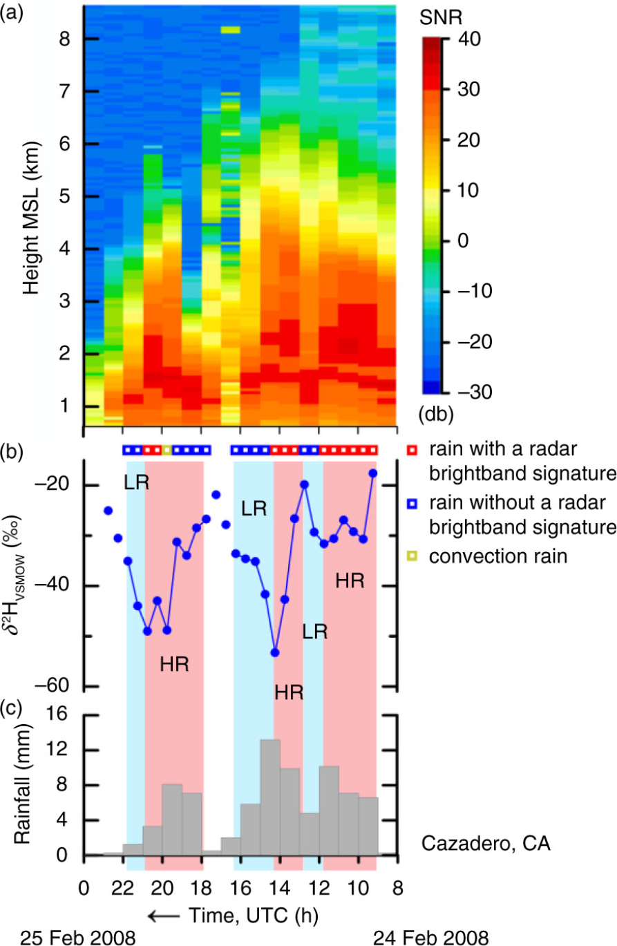
Fig. A10
(a) Time–height section of equivalent radar reflectivity factor with signal-to-noise ratio (SNR), (b) time series of δ 2HVSMOW values of 30-min, time-integrated precipitation samples and (c) histogram of hourly rainfall at Cazadero, CA, collected between 8 UTC 24 February 2008 and 0 UTC 25 February 2008. HR, pink panels, higher rainout, decreasing or low δ 2HVSMOW values. LR, blue panels, lower rainout, increasing or high δ 2HVSMOW values. Open squares indicate objective categorization of the rainfall occurring during selected half-hour periods. Time increases from right to left.
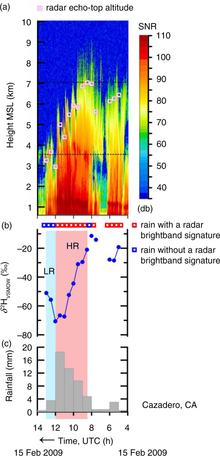
Fig. A11
(a) Time–height section of equivalent radar reflectivity factor with signal-to-noise ratio (SNR), (b) time series of δ 2HVSMOW values of 30-min, time-integrated precipitation samples and (c) histogram of hourly rainfall at Cazadero, CA, collected between 4 and 14 UTC 15 February 2009. Open magenta squares indicate echo-top height. HR, pink panel, higher rainout, decreasing or low δ 2HVSMOW values. LR, blue panel, lower rainout, increasing or high δ 2HVSMOW values. Open squares indicate objective categorization of the rainfall occurring during selected half-hour periods. Dashed horizontal lines are KMUX NEXRAD 0.5-degree beam. Time increases from right to left.
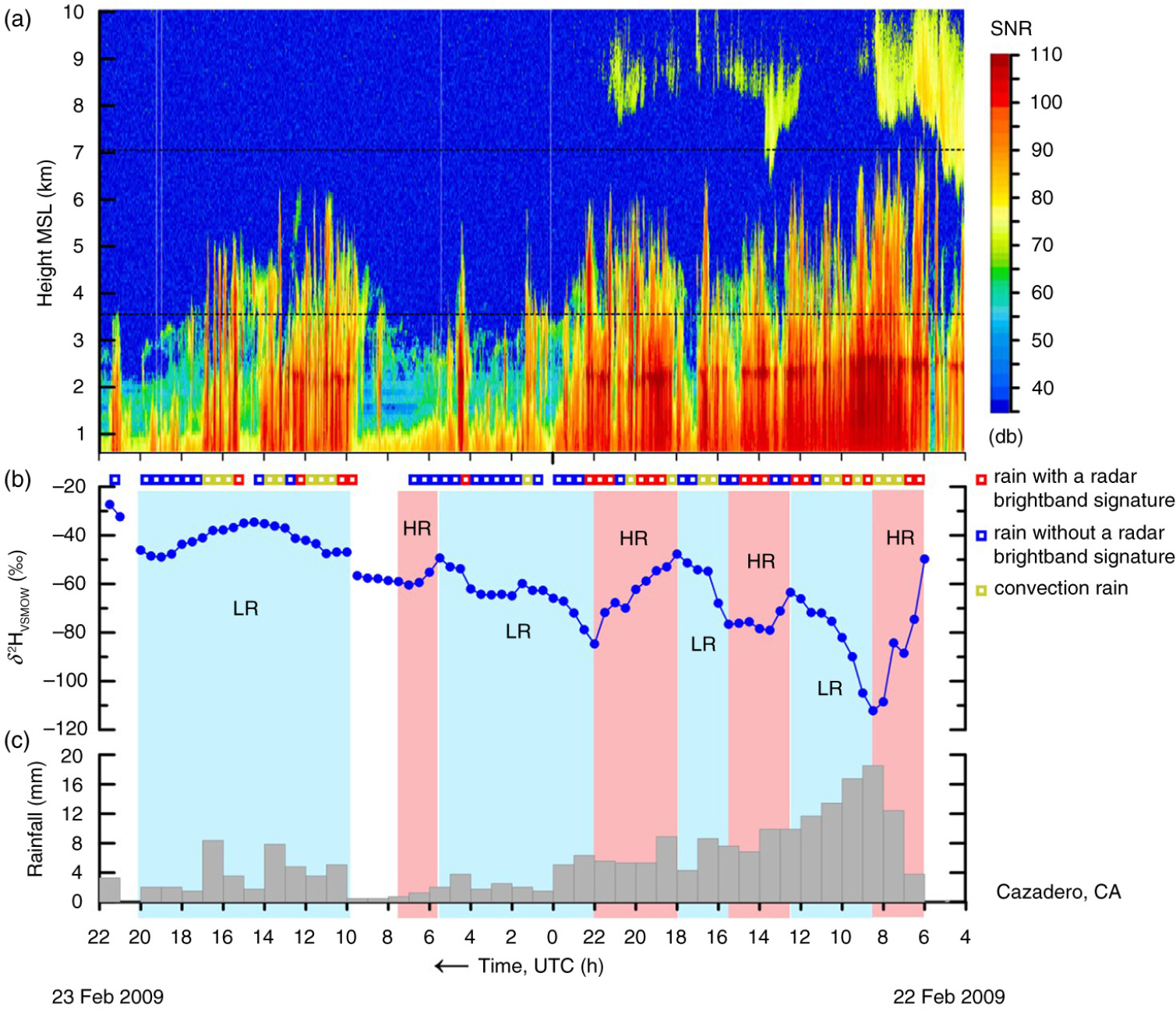
Fig. A12
(a) Time–height section of equivalent radar reflectivity factor with signal-to-noise ratio (SNR), (b) time series of δ 2HVSMOW values of 30-min, time-integrated precipitation samples and (c) histogram of hourly rainfall at Cazadero, CA, collected between 4 UTC 22 February 2009 and 22 UTC 23 February 2009. HR, pink panels, higher rainout, decreasing or low δ 2HVSMOW values. LR, blue panels, lower rainout, increasing or high δ 2HVSMOW values. Open squares indicate objective categorization of the rainfall occurring during selected half-hour periods. Dashed horizontal lines are KMUX NEXRAD 0.5-degree beam. Time increases from right to left.
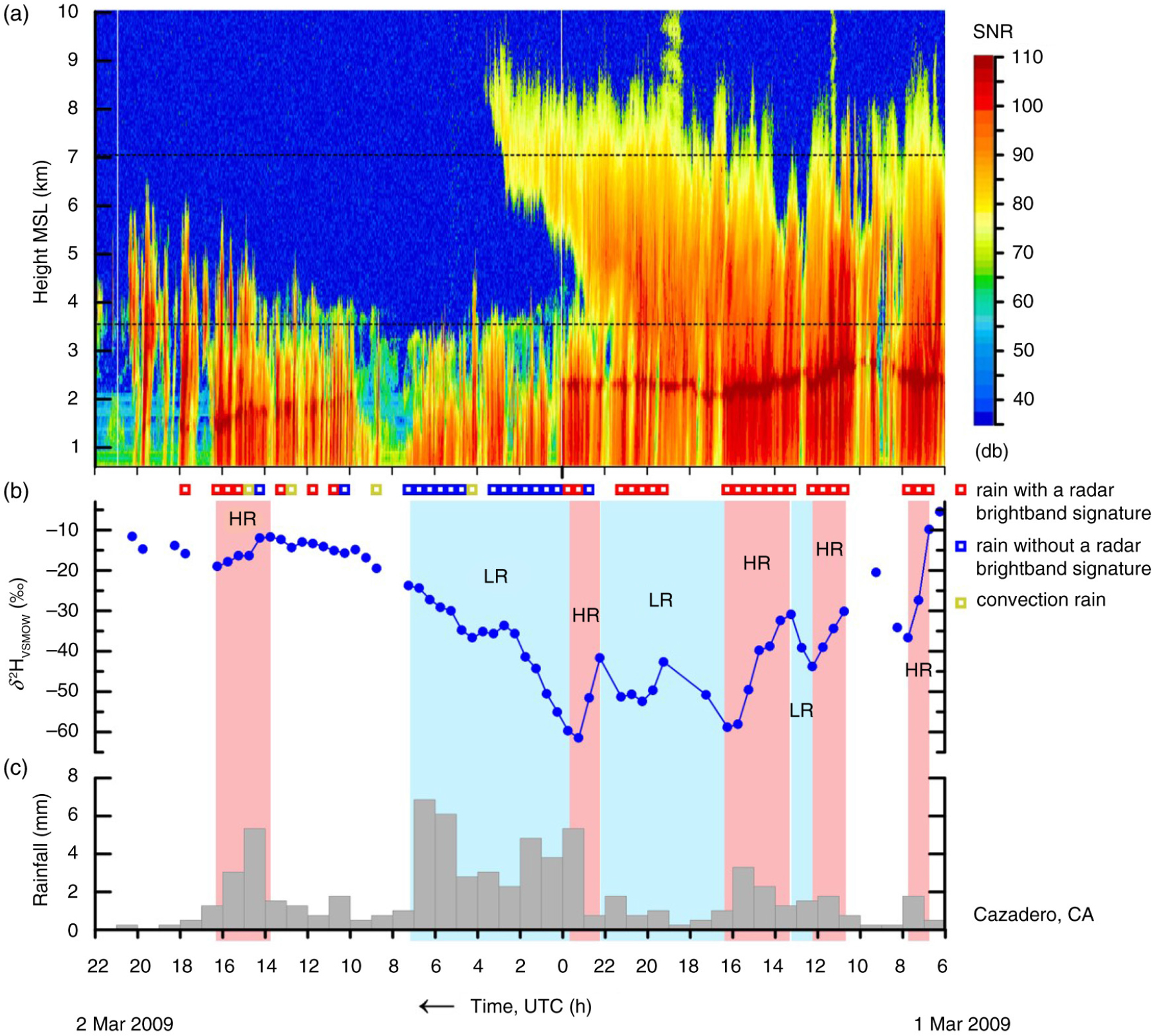
Fig. A13
(a) Time–height section of equivalent radar reflectivity factor with signal-to-noise ratio (SNR), (b) time series of δ 2HVSMOW values of 30-min, time-integrated precipitation samples and (c) histogram of hourly rainfall at Cazadero, CA, collected between 6 UTC 1 March 2009 and 22 UTC 2 March 2009. HR, pink panels, higher rainout, decreasing or low δ 2HVSMOW values. LR, blue panels, lower rainout, increasing or high δ 2HVSMOW values. Open squares indicate objective categorization of the rainfall occurring during selected half-hour periods. Dashed horizontal lines are KMUX NEXRAD 0.5-degree beam. Time increases from right to left.
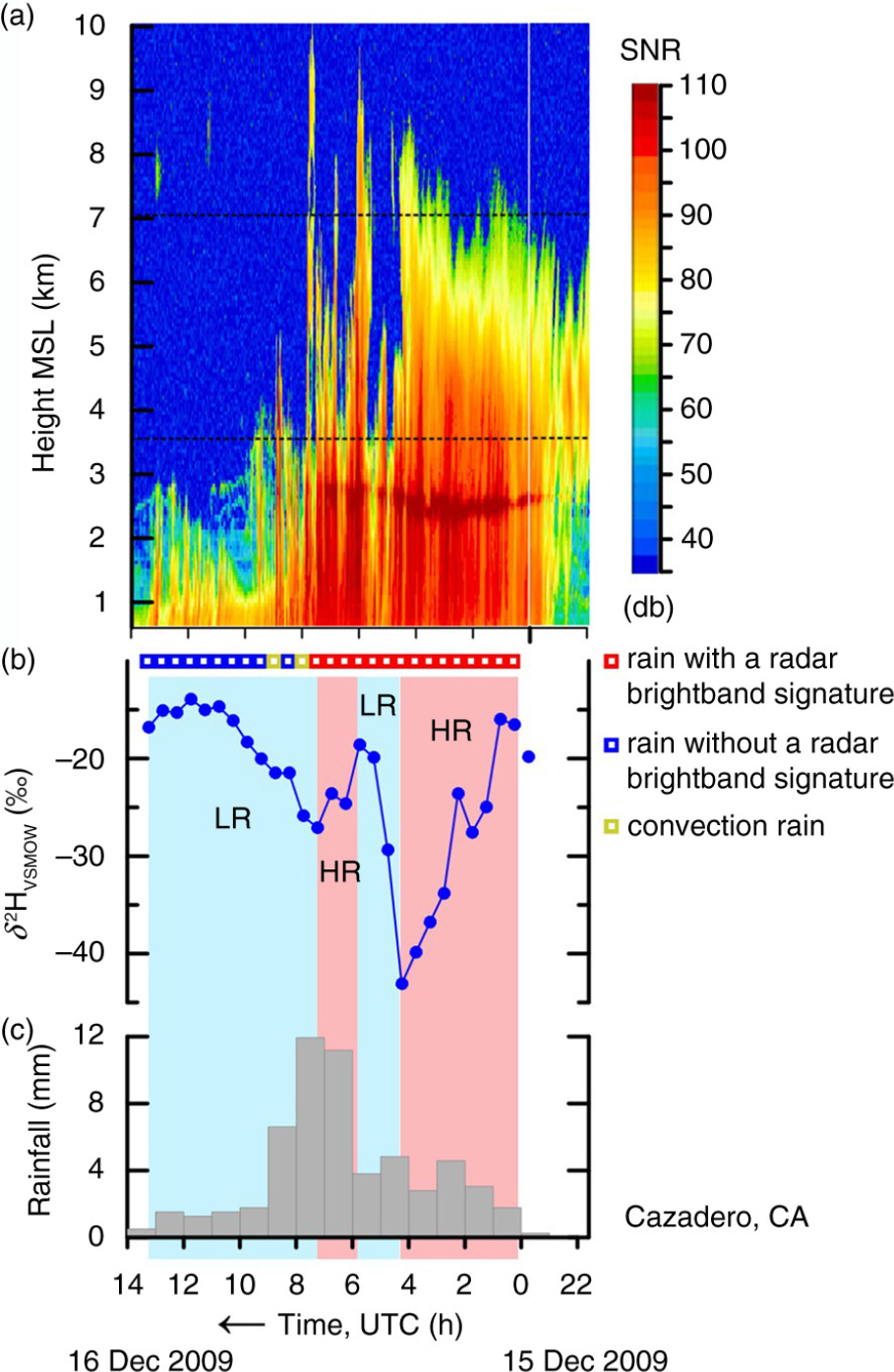
Fig. A14
(a) Time–height section of equivalent radar reflectivity factor with signal-to-noise ratio (SNR), (b) time series of δ 2HVSMOW values of 30-min, time-integrated precipitation samples and (c) histogram of hourly rainfall at Cazadero, CA, collected between 22 UTC 15 December 2009 and 14 UTC 16 December 2009. HR, pink panels, higher rainout, decreasing or low δ 2HVSMOW values. LR, blue panels, lower rainout, increasing or high δ 2HVSMOW values. Dashed horizontal lines are KMUX NEXRAD 0.5-degree beam. Time increases from right to left.
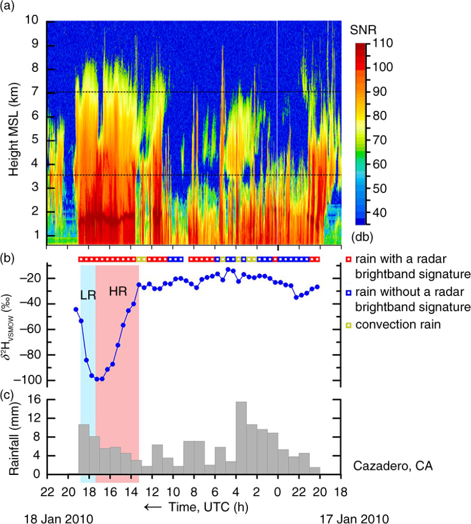
Fig. A15
(a) Time–height section of equivalent radar reflectivity factor with signal-to-noise ratio (SNR), (b) time series of δ 2HVSMOW values of 30-min, time-integrated precipitation samples and (c) histogram of hourly rainfall at Cazadero, CA, collected between 18 UTC 17 January 2010 and 22 UTC 18 January 2010. Open magenta squares indicate echo-top height. HR, pink panel, higher rainout, decreasing or low δ 2HVSMOW values. LR, blue panel, lower rainout, increasing or high δ 2HVSMOW values. Open squares indicate objective categorization of the rainfall occurring during selected half-hour periods. Dashed horizontal lines are KMUX NEXRAD 0.5-degree beam. Time increases from right to left.
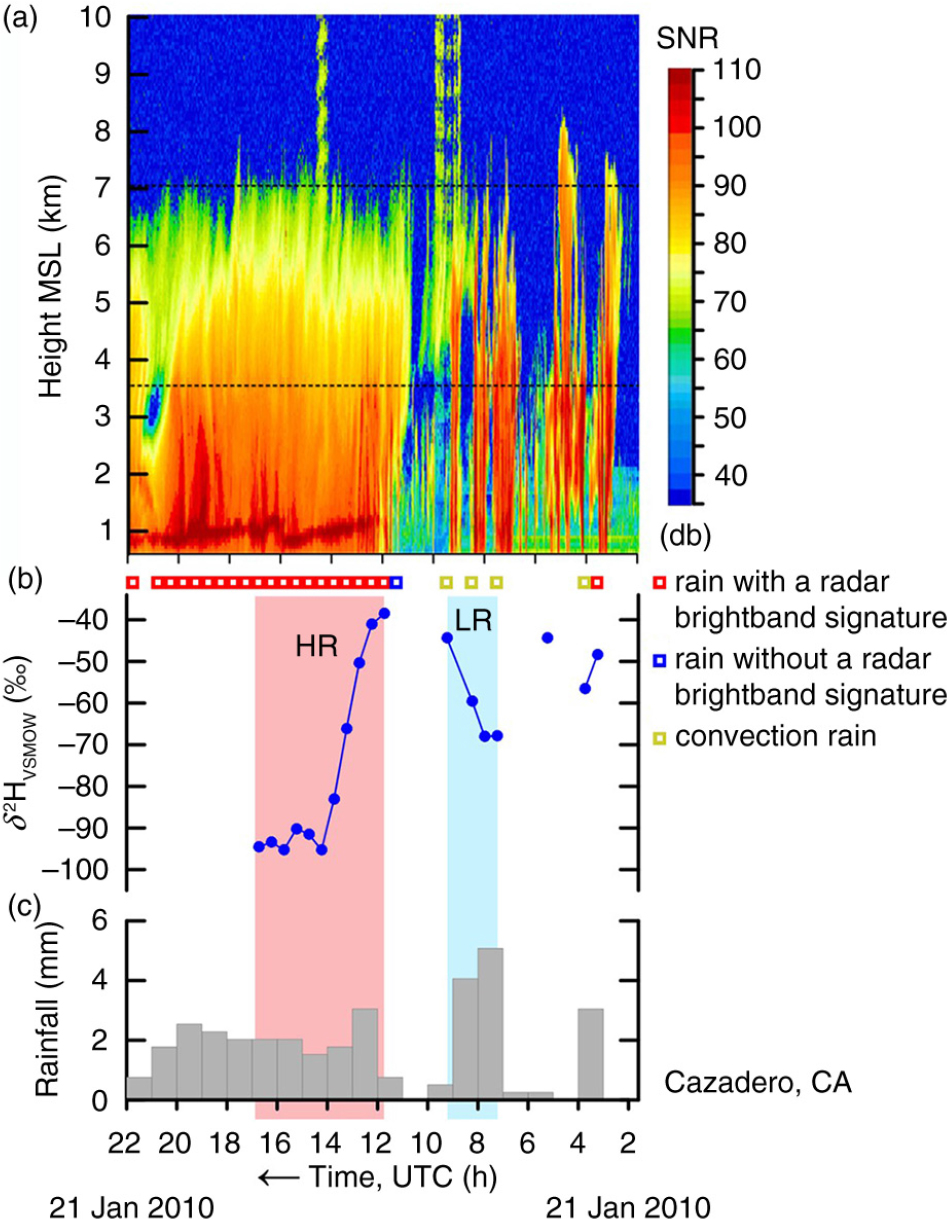
Fig. A16
(a) Time–height section of equivalent radar reflectivity factor with signal-to-noise ratio (SNR), (b) time series of δ 2HVSMOW values of 30-min, time-integrated precipitation samples and (c) histogram of hourly rainfall at Cazadero, CA, collected between 2 and 22 UTC 21 January 2010. HR, pink panel, higher rainout, decreasing or low δ 2HVSMOW values. LR, blue panel, lower rainout, increasing or high δ 2HVSMOW values. Open squares indicate objective categorization of the rainfall occurring during selected half-hour periods. Dashed horizontal lines are KMUX NEXRAD 0.5-degree beam. Time increases from right to left.
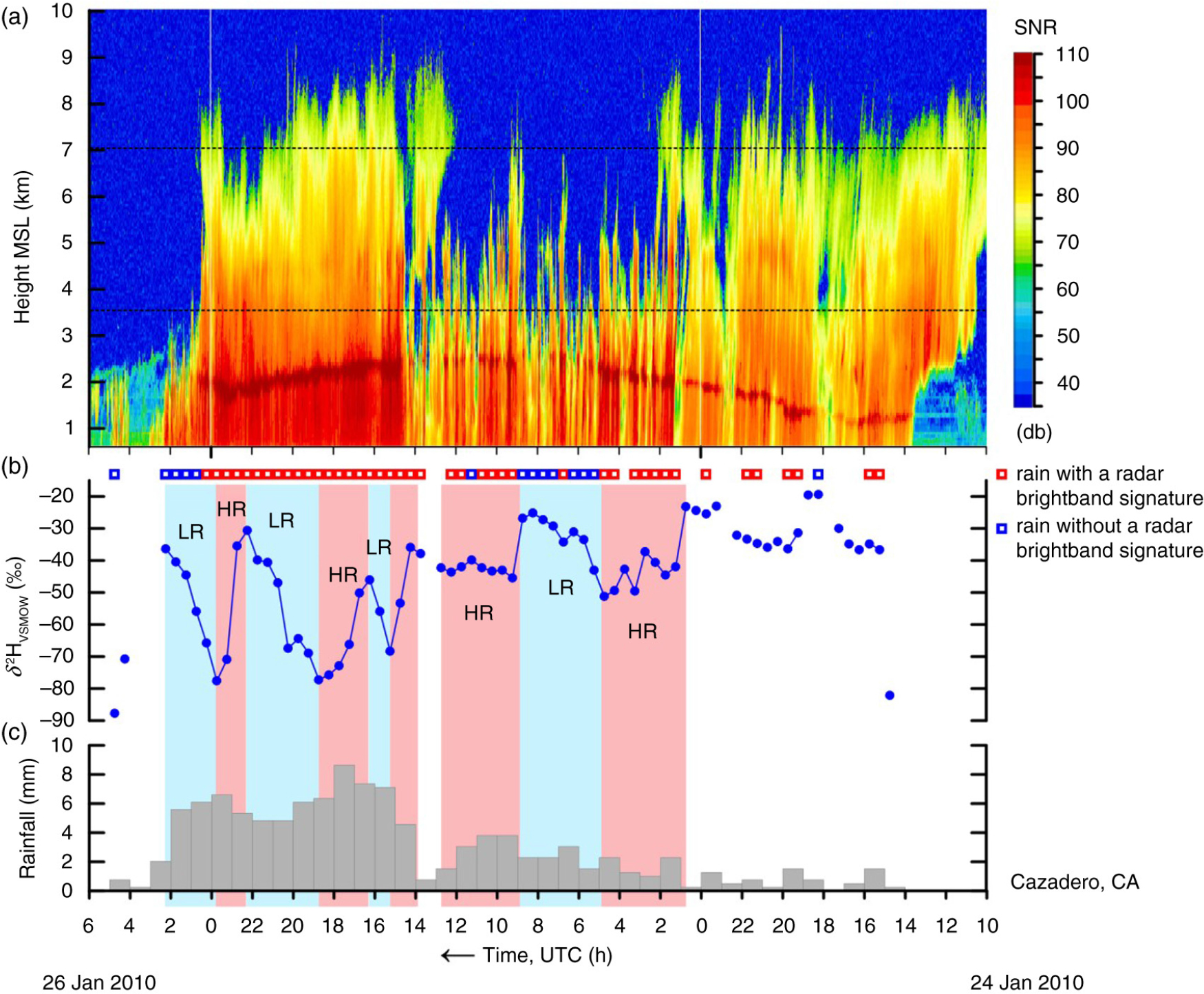
Fig. A17
(a) Time–height section of equivalent radar reflectivity factor with signal-to-noise ratio (SNR), (b) time series of δ 2HVSMOW values of 30-min, time-integrated precipitation samples and (c) histogram of hourly rainfall at Cazadero, CA, collected between 10 UTC 24 January 2010 and 6 UTC 26 January 2010. HR, pink panels, higher rainout, decreasing or low δ 2HVSMOW values. LR, blue panels, lower rainout, increasing or high δ 2HVSMOW values. Open squares indicate objective categorization of the rainfall occurring during selected half-hour periods. Dashed horizontal lines are KMUX NEXRAD 0.5-degree beam. Time increases from right to left.
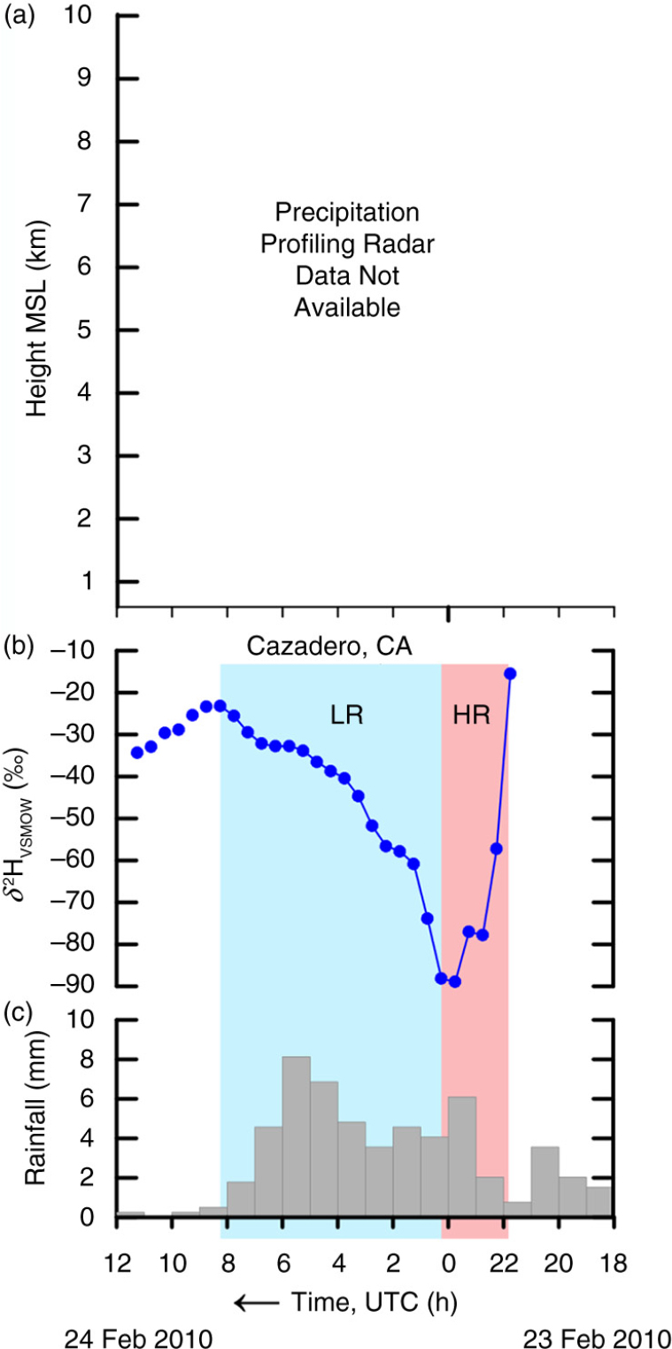
Fig. A18
(a) Time–height section of equivalent radar reflectivity factor with signal-to-noise ratio (SNR), (b) time series of δ 2HVSMOW values of 30-min, time-integrated precipitation samples and (c) histogram of hourly rainfall at Cazadero, CA, collected between 18 UTC 23 February 2010 and 12 UTC 24 February 2010. Period HR, pink panel, higher rainout, decreasing or low δ 2HVSMOW values. LR, blue panel, lower rainout, increasing or high δ 2HVSMOW values. Time increases from right to left.
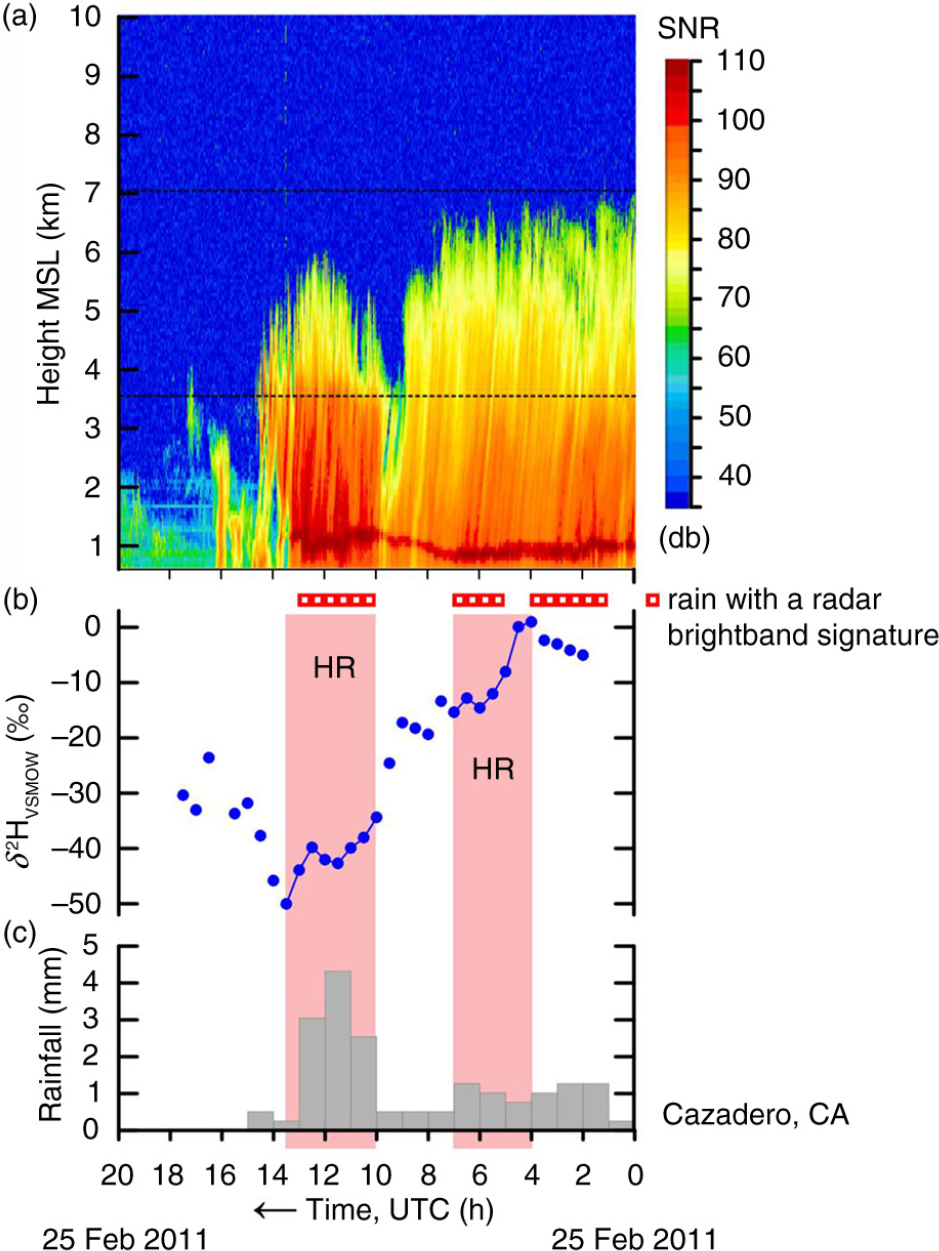
Fig. A19
(a) Time–height section of equivalent radar reflectivity factor with signal-to-noise ratio (SNR), (b) time series of δ 2HVSMOW values of 30-min, time-integrated precipitation samples and (c) histogram of hourly rainfall at Cazadero, CA, collected between 0 and 20 UTC 25 February 2011. HR, pink panels, higher rainout, decreasing or low δ 2HVSMOW values. Open squares indicate objective categorization of the rainfall occurring during selected half-hour periods. Dashed horizontal lines are KMUX NEXRAD 0.5-degree beam. Time increases from right to left.
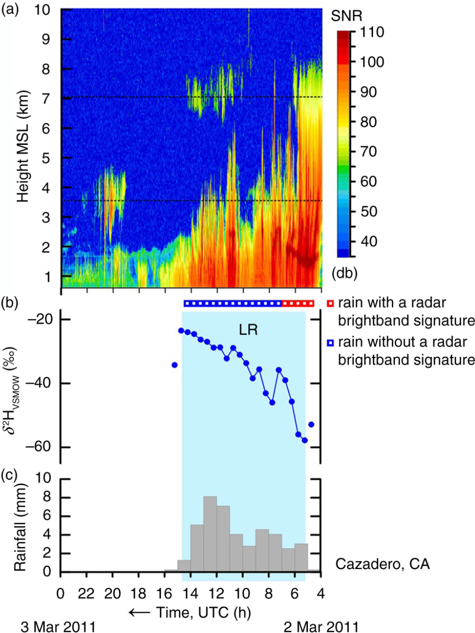
Fig. A20
(a) Time–height section of equivalent radar reflectivity factor with signal-to-noise ratio (SNR), (b) time series of δ 2HVSMOW values of 30-min, time-integrated precipitation samples and (c) histogram of hourly rainfall at Cazadero, CA, collected between 4 UTC 2 March 2011 and 0 UTC 3 March 2011. LR, blue panel, lower rainout, increasing or high δ 2HVSMOW values. Open squares indicate objective categorization of the rainfall occurring during selected half-hour periods. Dashed horizontal lines are KMUX NEXRAD 0.5-degree beam. Time increases from right to left. The date–time value of the first sample is estimated within ±2 h. The date–time values of the other samples are precise to within ±1 min relative to the first sample.
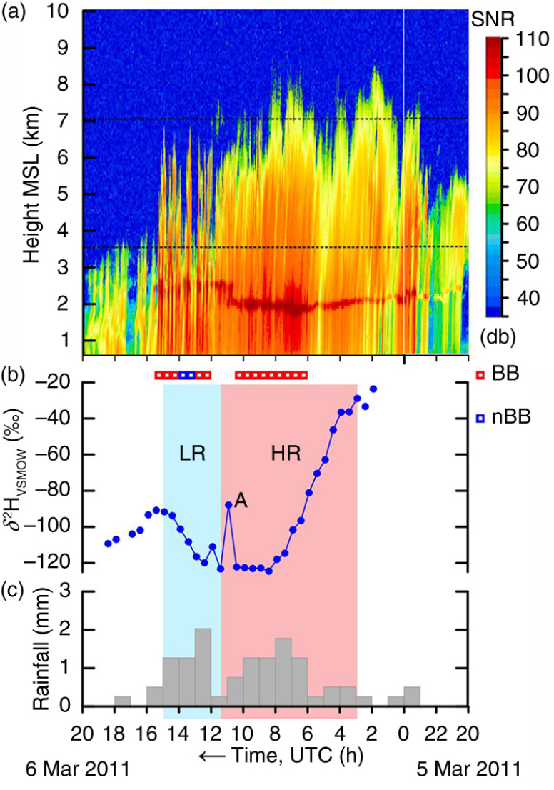
Fig. A21
(a) Time–height section of equivalent radar reflectivity factor with signal-to-noise ratio (SNR), (b) time series of δ 2HVSMOW values of 30-min, time-integrated precipitation samples and (c) histogram of hourly rainfall at Cazadero, CA, collected between 20 UTC 5 March 2011 and 20 UTC 6 March 2011. HR, pink panel, higher rainout, decreasing or low δ 2HVSMOW values. LR, blue panel, lower rainout, increasing or high δ 2HVSMOW values. Open squares indicate objective categorization of the rainfall occurring during selected half-hour periods. Dashed horizontal lines are KMUX NEXRAD 0.5-degree beam. Time increases from right to left. The date–time value of the first sample is estimated within ±2 h. The date–time values of the other samples are precise to within ±1 min relative to the first sample.
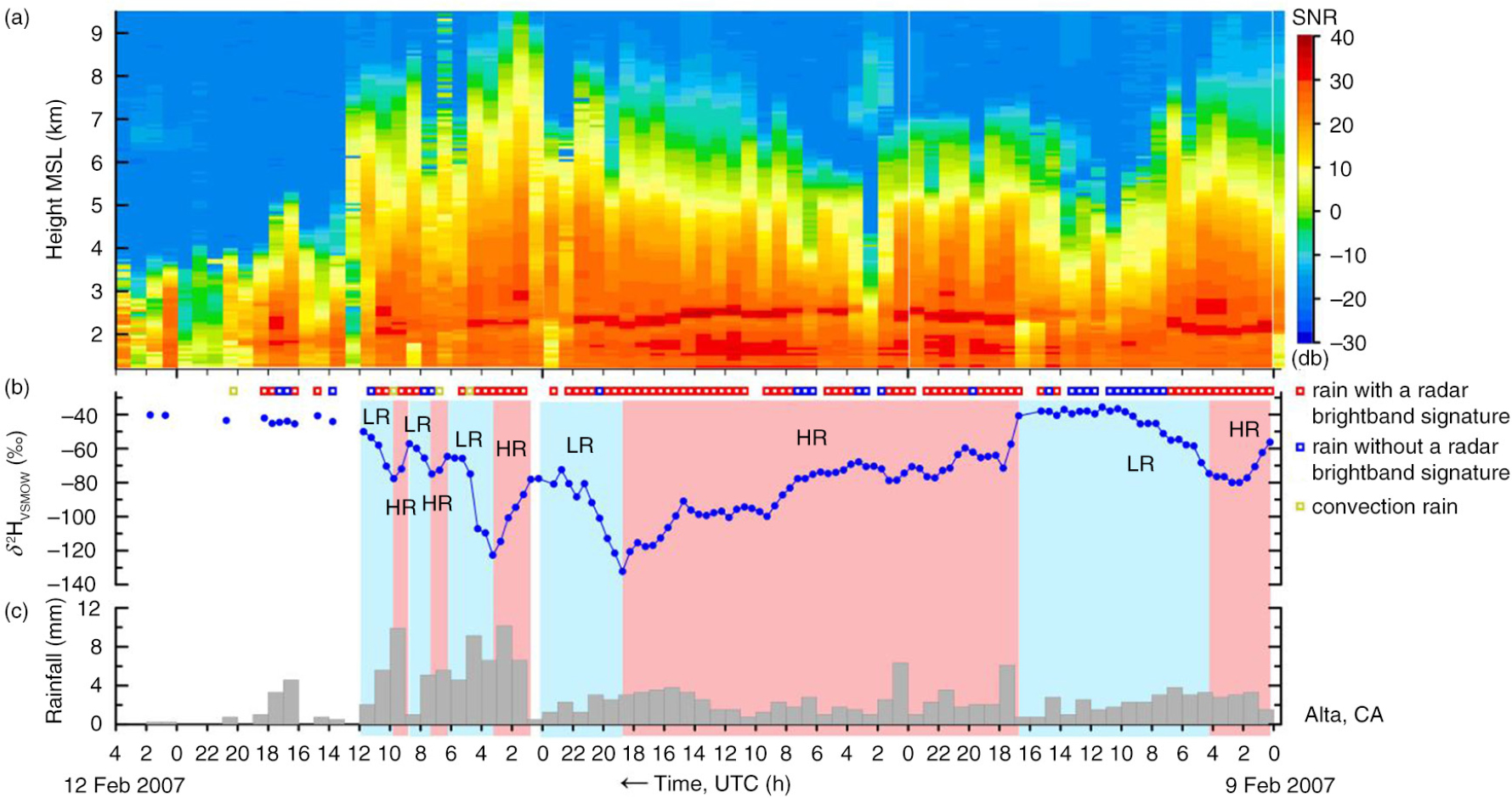
Fig. A22
(a) Time–height section of equivalent radar reflectivity factor with signal-to-noise ratio (SNR), (b) time series of δ 2HVSMOW values of 30-min, time-integrated precipitation samples and (c) histogram of hourly rainfall at Alta, CA, collected between 0 UTC 9 February 2007 and 4 UTC 12 February 2007. HR, pink panels, higher rainout, decreasing or low δ 2HVSMOW values. LR, blue panels, lower rainout, increasing or high δ 2HVSMOW values. Open squares indicate objective categorization of the rainfall occurring during selected half-hour periods. Time increases from right to left.
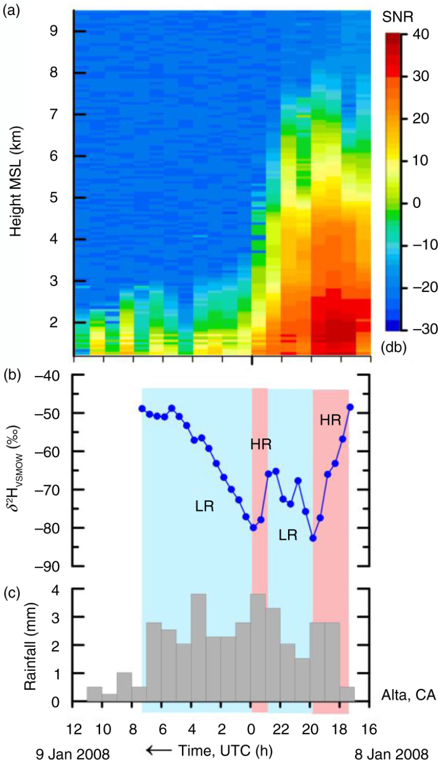
Fig. A23
(a) Time–height section of equivalent radar reflectivity factor with signal-to-noise ratio (SNR), (b) time series of δ 2HVSMOW values of 30-min, time-integrated precipitation samples and (c) histogram of hourly rainfall at Alta, CA, collected between 16 UTC 8 January 2008 and 12 UTC 9 January 2008. HR, pink panels, higher rainout, decreasing or low δ 2HVSMOW values. LR, blue panels, lower rainout, increasing or high δ 2HVSMOW values. Time increases from right to left.
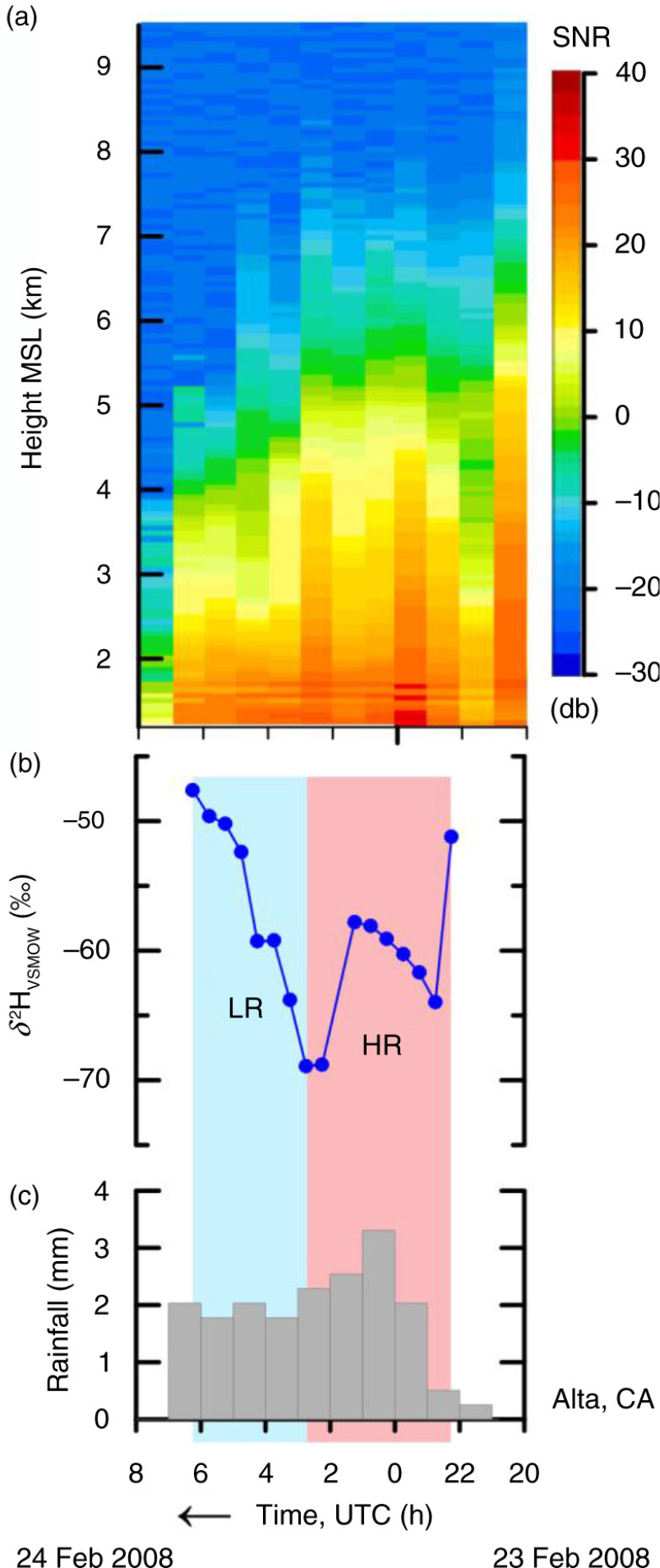
Fig. A24
(a) Time–height section of equivalent radar reflectivity factor with signal-to-noise ratio (SNR), (b) time series of δ 2HVSMOW values of 30-min, time-integrated precipitation samples and (c) histogram of hourly rainfall at Alta, CA, collected between 20 UTC 23 February 2008 and 8 UTC 24 February 2008. HR, pink panel, higher rainout, decreasing or low δ 2HVSMOW values. LR, blue panel, lower rainout, increasing or high δ 2HVSMOW values. Time increases from right to left.
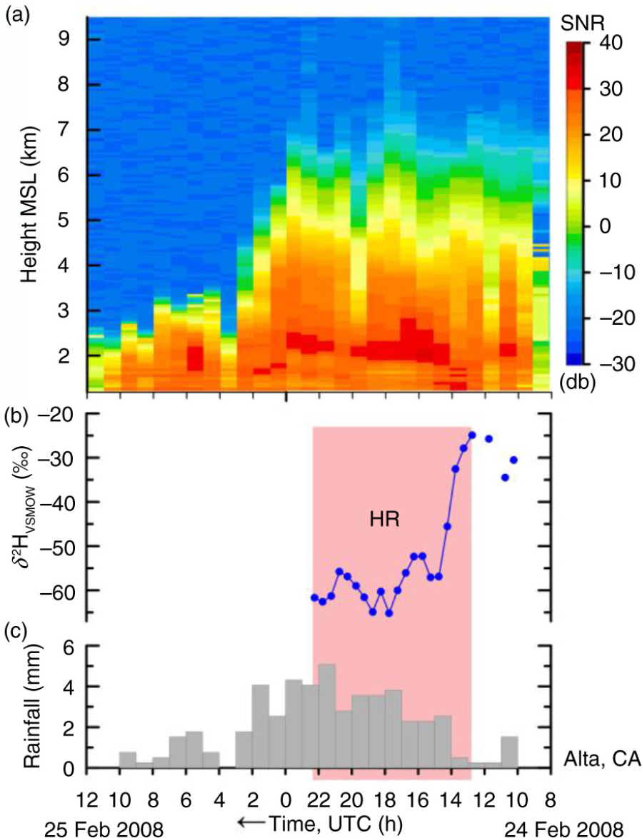
Fig. A25
(a) Time–height section of equivalent radar reflectivity factor with signal-to-noise ratio (SNR), (b) time series of δ 2HVSMOW values of 30-min, time-integrated precipitation samples and (c) histogram of hourly rainfall at Alta, CA, collected between 8 UTC 24 February 2008 and 12 UTC 25 February 2008. HR, pink panel, higher rainout, decreasing or low δ 2HVSMOW values. Time increases from right to left. No samples were collected after 23 UTC 24 February 2008 owing to collector-power problems.
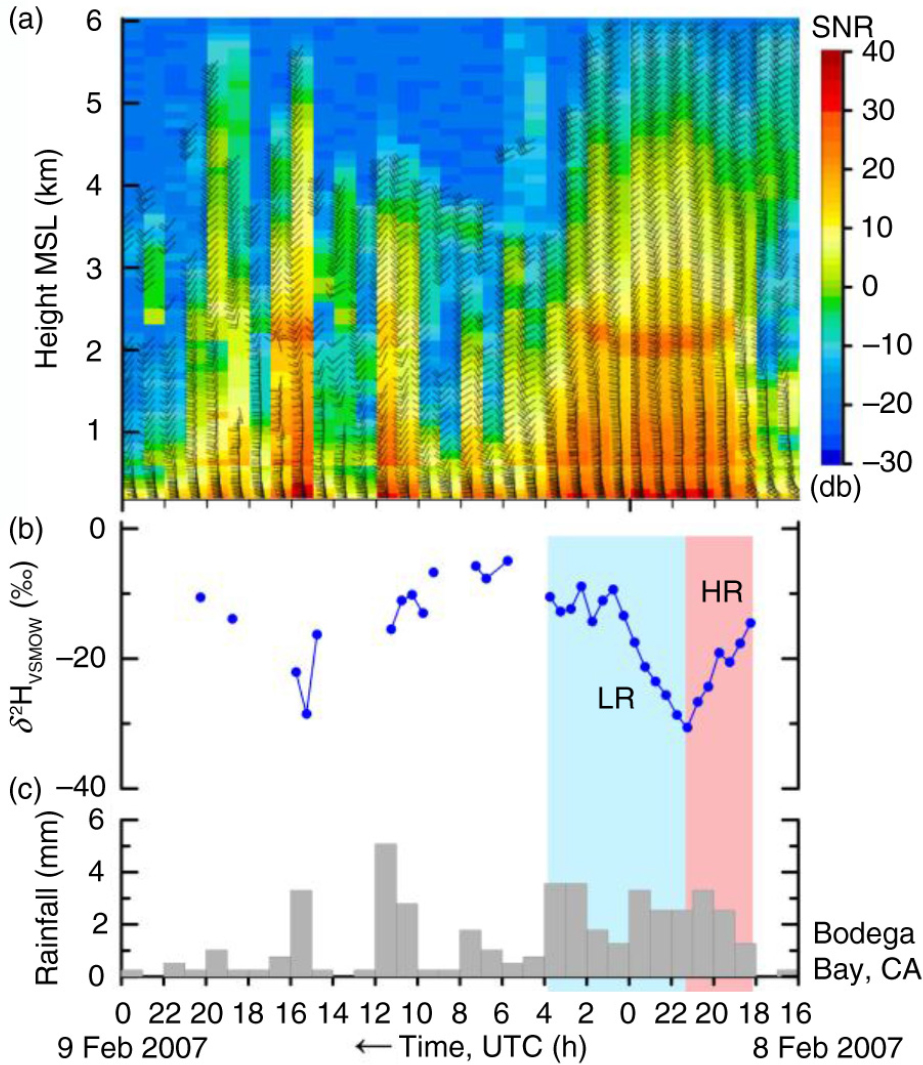
Fig. A26
(a) Time–height series of hourly wind profiles (flags: 25 m s−1; barbs: 5 m s−1; half-barbs: 2.5 m s−1) with signal-to-noise ratio (SNR), (b) time series of δ 2HVSMOW values of 30-min, time-integrated precipitation samples and (c) histogram of hourly rainfall at Bodega Bay, CA, collected between 16 UTC 8 February 2007 and 0 UTC 9 February 2007. HR, pink panel, higher rainout, decreasing or low δ 2HVSMOW values. LR, blue panel, lower rainout, increasing or high δ 2HVSMOW values. Time increases from right to left.
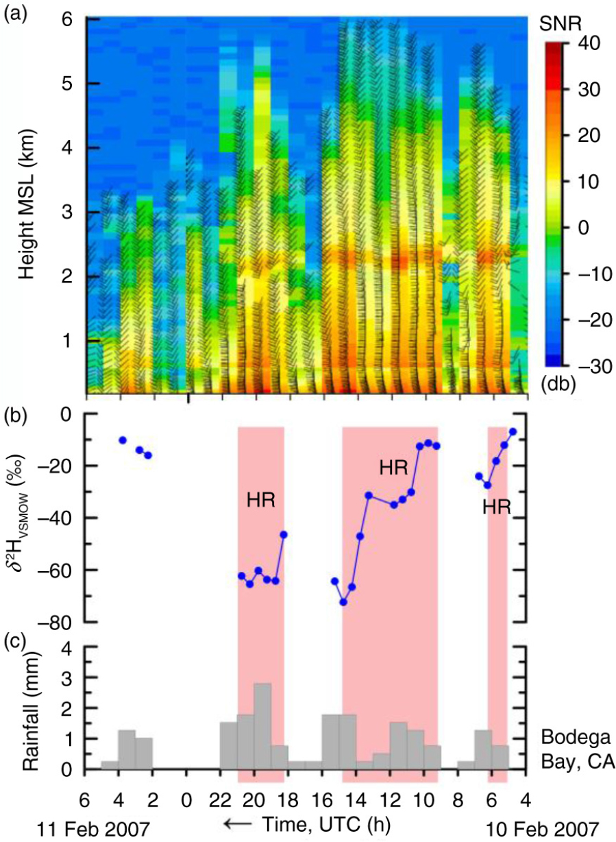
Fig. A27
(a) Time–height series of hourly wind profiles (flags: 25 m s−1; barbs: 5 m s−1; half-barbs: 2.5 m s−1) with signal-to-noise ratio (SNR), (b) time series of δ 2HVSMOW values of 30-min, time-integrated precipitation samples and (c) histogram of hourly rainfall at Bodega Bay, CA, collected between 4 UTC 10 February 2007 and 6 UTC 11 February 2007. HR, pink panels, higher rainout, decreasing or low δ 2HVSMOW values. Time increases from right to left.
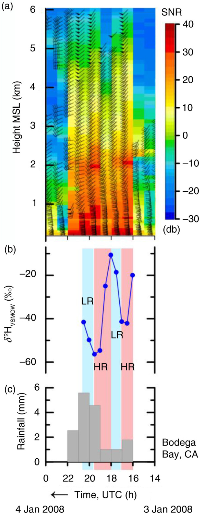
Fig. A28
(a) Time–height series of hourly wind profiles (flags: 25 m s−1; barbs: 5 m s−1; half-barbs: 2.5 m s−1) with signal-to-noise ratio (SNR), (b) time series of δ 2HVSMOW values of 30-min, time-integrated precipitation samples and (c) histogram of hourly rainfall at Bodega Bay, CA, collected between 14 UTC 3 January 2008 and 0 UTC 4 January 2008. HR, pink panels, higher rainout, decreasing or low δ 2HVSMOW values. LR, blue panels, lower rainout, increasing or high δ 2HVSMOW values. Time increases from right to left.
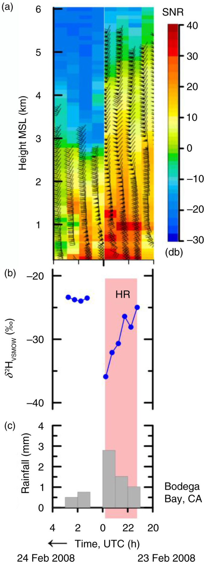
Fig. A29
(a) Time–height series of hourly wind profiles (flags: 25 m s−1; barbs: 5 m s−1; half-barbs: 2.5 m s−1) with signal-to-noise ratio (SNR), (b) time series of δ 2HVSMOW values of 30-min, time-integrated precipitation samples and (c) histogram of hourly rainfall at Bodega Bay, CA, collected between 20 UTC 23 February 2008 and 4 UTC 24 February 2008. HR, pink panel, higher rainout, decreasing or low δ 2HVSMOW values. Time increases from right to left.
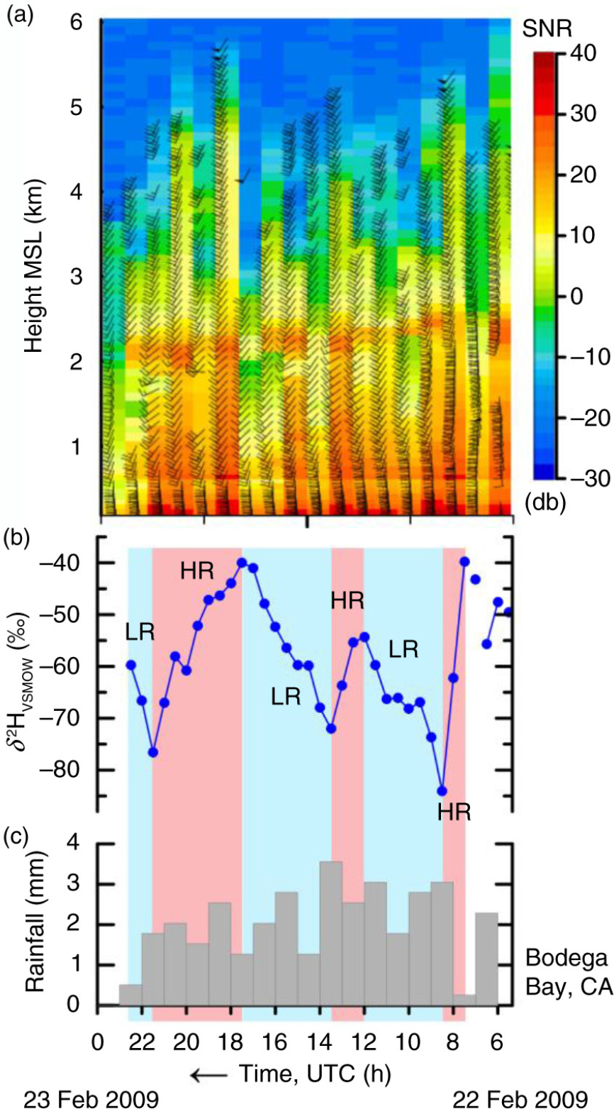
Fig. A30
(a) Time–height series of hourly wind profiles (flags: 25 m s−1; barbs: 5 m s−1; half-barbs: 2.5 m s−1) with signal-to-noise ratio (SNR), (b) time series of δ 2HVSMOW values of 30-min, time-integrated precipitation samples and (c) histogram of hourly rainfall at Bodega Bay, CA, collected between 6 UTC 22 February 2009 and 0 UTC 23 February 2009. HR, pink panels, higher rainout, decreasing or low δ 2HVSMOW values. LR, blue panels, lower rainout, increasing or high δ 2HVSMOW values. Time increases from right to left.
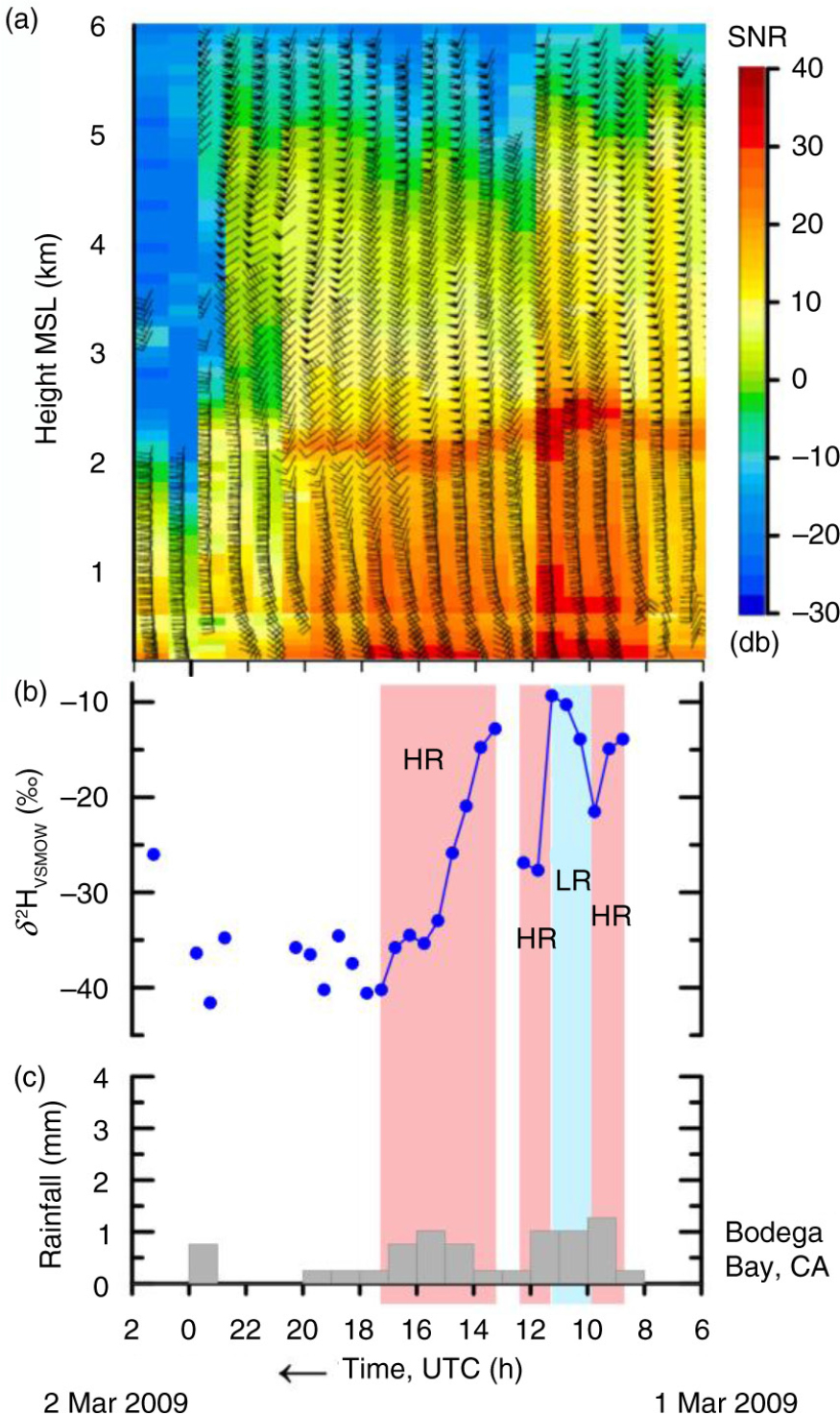
Fig. A31
(a) Time–height series of hourly wind profiles (flags: 25 m s−1; barbs: 5 m s−1; half-barbs: 2.5 m s−1) with signal-to-noise ratio (SNR), (b) time series of δ 2HVSMOW values of 30-min, time-integrated precipitation samples and (c) histogram of hourly rainfall at Bodega Bay, CA, collected between 6 UTC 1 March 2009 and 2 UTC 2 March 2009. HR, pink panels, higher rainout, decreasing or low δ 2HVSMOW values. LR, blue panel, lower rainout, increasing or high δ 2HVSMOW values. Time increases from right to left.
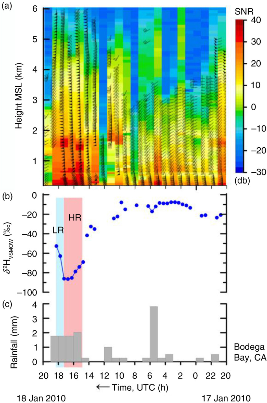
Fig. A32
(a) Time–height series of hourly wind profiles (flags: 25 m s−1; barbs: 5 m s−1; half-barbs: 2.5 m s−1) with signal-to-noise ratio, NR, (b) time series of δ 2HVSMOW values of 30-min, time-integrated precipitation samples and (c) histogram of hourly rainfall at Bodega Bay, CA, collected between 20 UTC 17 January 2010 and 20 UTC 18 January 2010. HR, pink panel, higher rainout, decreasing or low δ 2HVSMOW values. LR, blue panel, lower rainout, increasing or high δ 2HVSMOW values. Time increases from right to left.
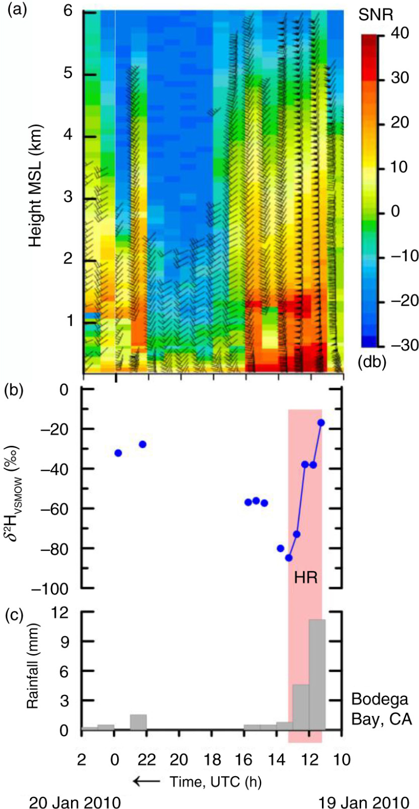
Fig. A33
(a) Time–height series of hourly wind profiles (flags: 25 m s−1; barbs: 5 m s−1; half-barbs: 2.5 m s−1) with signal-to-noise ratio, (SNR), (b) time series of δ 2HVSMOW values of 30-min, time-integrated precipitation samples and (c) histogram of hourly rainfall at Bodega Bay, CA, collected between 10 UTC 19 January 2010 and 2 UTC 20 January 2010. HR, pink panel, higher rainout, decreasing or low δ 2HVSMOW values. Time increases from right to left.
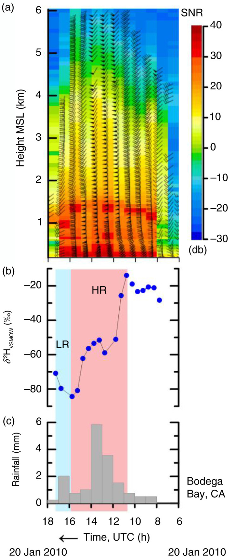
Fig. A34
(a) Time–height series of hourly wind profiles (flags: 25 m s−1; barbs: 5 m s−1; half-barbs: 2.5 m s−1) with signal-to-noise ratio (SNR), (b) time series of δ 2HVSMOW values of 30-min, time-integrated precipitation samples and (c) histogram of hourly rainfall at Bodega Bay, CA, collected between 6 and 18 UTC 20 January 2010. HR, pink panel, higher rainout, decreasing or low δ 2HVSMOW values. LR, blue panel, lower rainout, increasing or high δ 2HVSMOW values. Time increases from right to left.
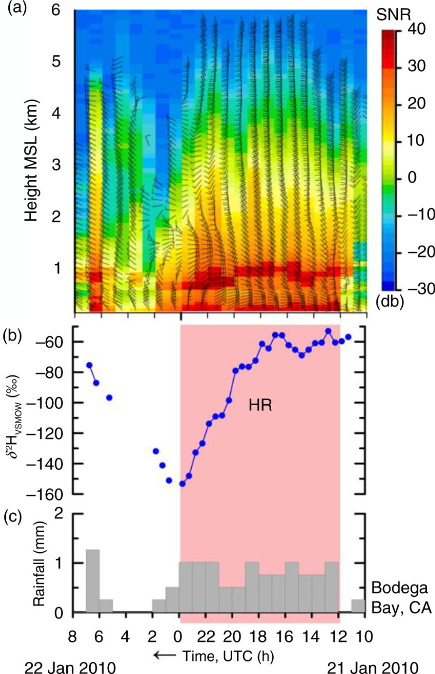
Fig. A35
(a) Time–height series of hourly wind profiles (flags: 25 m s−1; barbs: 5 m s−1; half-barbs: 2.5 m s−1) with signal-to-noise ratio (SNR), (b) time series of δ 2HVSMOW values of 30-min, time-integrated precipitation samples and (c) histogram of hourly rainfall at Bodega Bay, CA, collected between 10 UTC 21 January 2010 and 8 UTC 22 January 2010. HR, pink panel, higher rainout, decreasing or low δ 2HVSMOW values. Time increases from right to left.
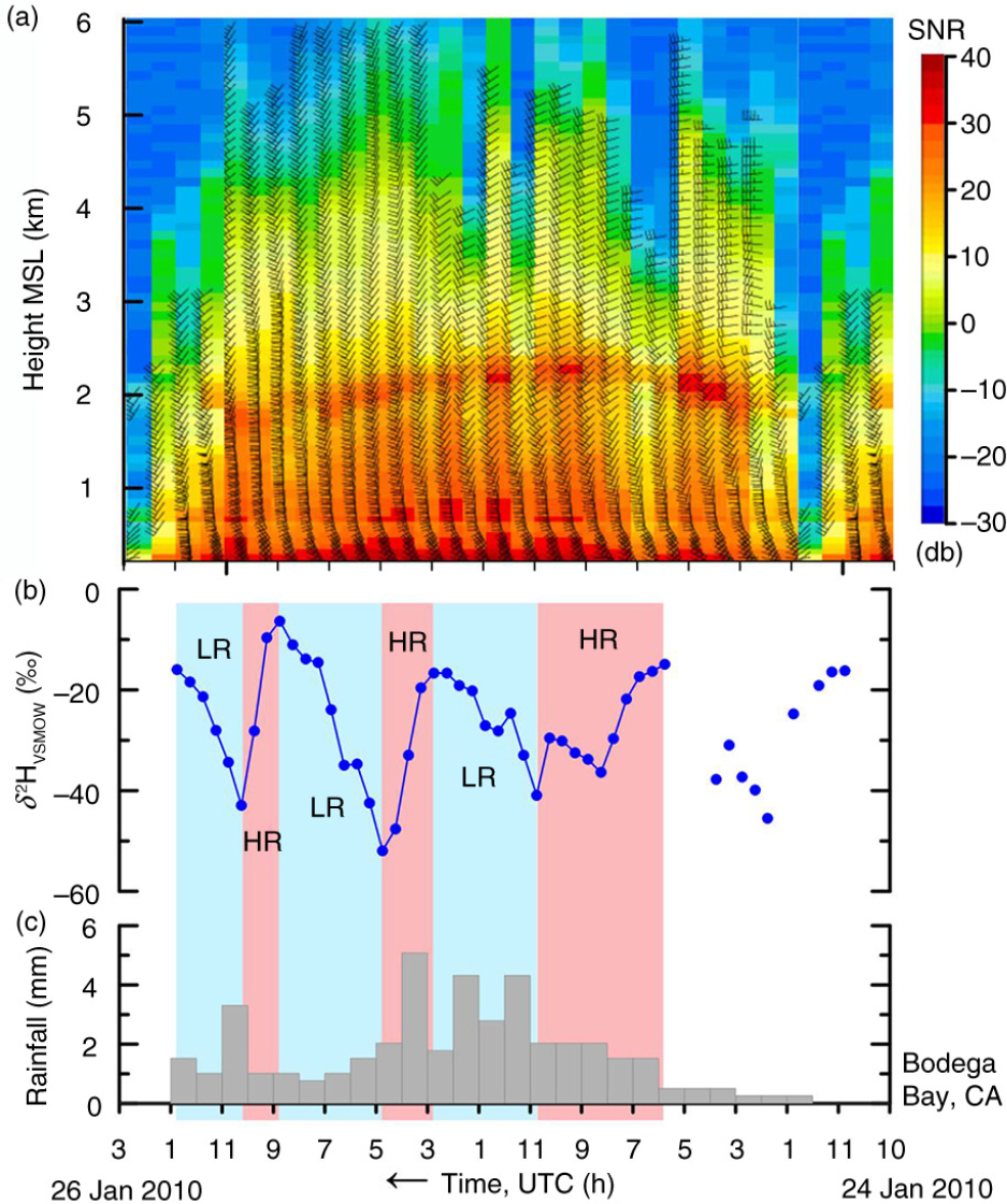
Fig. A36
(a) Time–height series of hourly wind profiles (flags: 25 m s−1; barbs: 5 m s−1; half-barbs: 2.5 m s−1) with signal-to-noise ratio (SNR), (b) time series of δ 2HVSMOW values of 30-min, time-integrated precipitation samples and (c) histogram of hourly rainfall at Bodega Bay, CA, collected between 22 UTC 24 January 2010 and 4 UTC 26 January 2010. HR, pink panels, higher rainout, decreasing or low δ 2HVSMOW values. LR, blue panels, lower rainout, increasing or high δ 2HVSMOW values. Time increases from right to left.
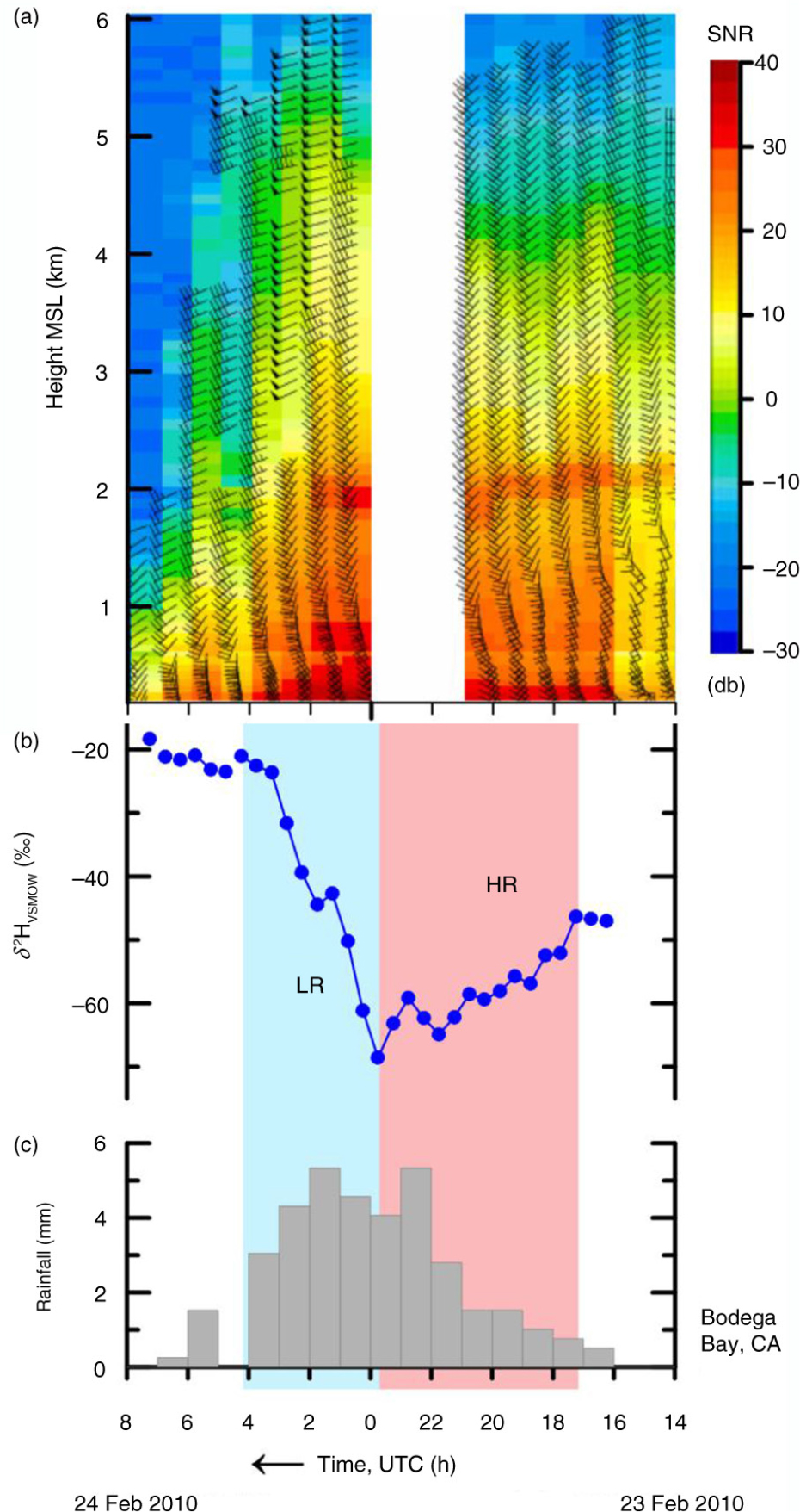
Fig. A37
(a) Time–height series of hourly wind profiles (flags: 25 m s−1; barbs: 5 m s−1; half-barbs: 2.5 m s−1) with signal-to-noise ratio (SNR), (b) time series of δ 2HVSMOW values of 30-min, time-integrated precipitation samples and (c) histogram of hourly rainfall at Bodega Bay, CA, collected between 14 UTC 23 February 2010 and 8 UTC 24 February 2010. HR, pink panel, higher rainout, decreasing or low δ 2HVSMOW values. LR, blue panel, lower rainout, increasing or high δ 2HVSMOW values. During a 3-hour period (21 UTC 23 February 2010 to 0 UTC 24 February 2010) wind-profiling data were not acquired. Time increases from right to left.
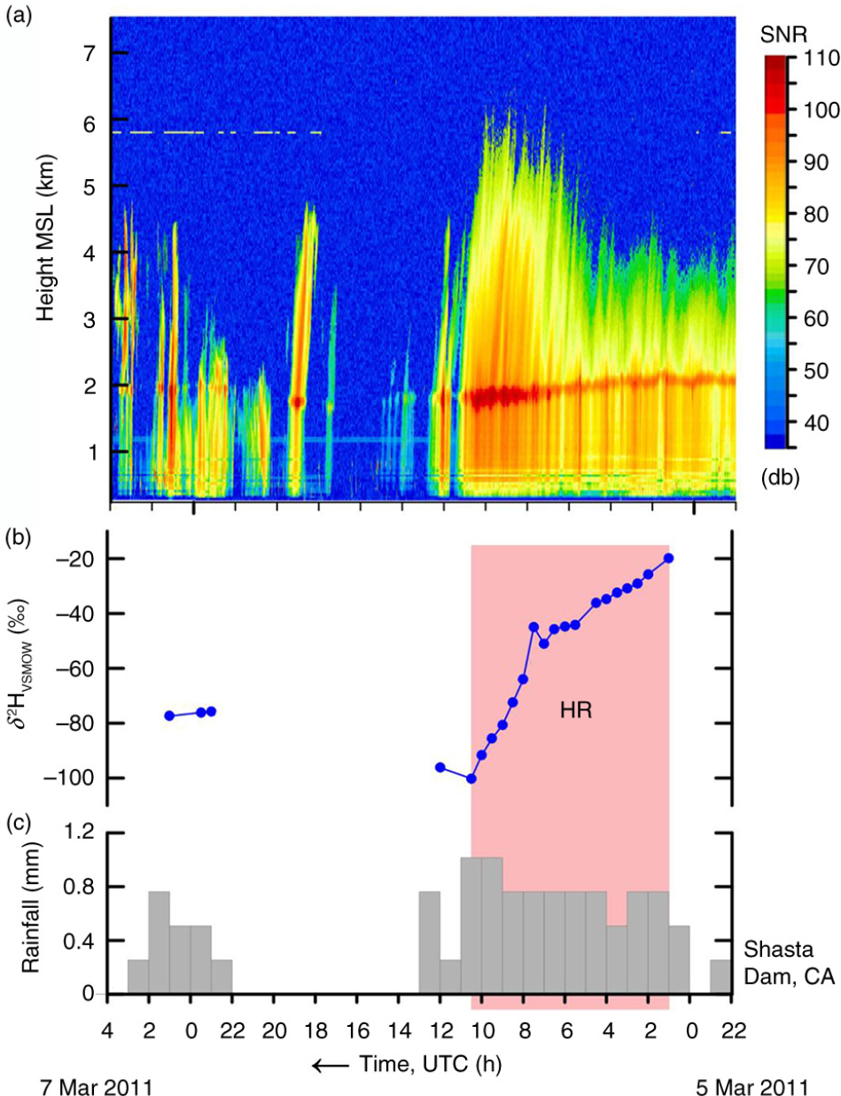
Fig. A38
(a) Time–height section of equivalent radar reflectivity factor with signal-to-noise ratio (SNR), (b) time series of δ 2HVSMOW values of 30-min, time-integrated precipitation samples and (c) histogram of hourly rainfall at Shasta Dam, CA, collected between 22 UTC 5 March 2011 and 4 UTC 7 March 2011. HR, pink panel, higher rainout, decreasing or low δ 2HVSMOW values. Time increases from right to left.
5. Summary and conclusions
With landfall of extratropical cyclones between January 2005 and March 2011, nearly 1400 precipitation samples were collected at four NOAA sites in California (ATA, BBY, CZD and STD) with novel automated sequential, time-integrating precipitation collectors. Samples from 43 events were collected and analysed for stable hydrogen and oxygen isotopic composition. Substantial decreases commonly were followed hours later by substantial increases in δ 2HVSMOW and δ 18OVSMOW of precipitation as pre-cold frontal precipitation generation transitioned from marine vapour masses having low rainout, to cold cloud layers having much higher rainout (with S-Prof BB signatures and lower δ 2HVSMOW values of precipitation), and finally to shallower, warmer precipitating clouds having lower rainout (with NBB signatures and higher δ 2HVSMOW values of precipitation), in accord with seeder–feeder precipitation. Decreases in δ 2HVSMOW of precipitation (the seeder portion of seeder–feeder precipitation) were identified in 82 intervals in these 43 events, ranging from 7.3 to a remarkable decrease of 100.5 ‰ for a 21 January 2010 event at BBY. The mean minimum δ 2HVSMOW value of rainfall is lower for landfalling ARs (−92.8 ‰, n=15) than that of non-AR extratropical cyclones (−65.2 ‰, n=16). The lowest δ 2HVSMOW value of rainfall from 29 CZD events was the exceptional value of −137.9 ‰ for the AR of 16 February 2009, suggesting involvement of relatively cold, deep clouds. All CZD events having δ 2HVSMOW values of rainfall below −105 ‰ were ARs (Fig. 17). Of the 13 events having δ 2HVSMOW values of rainfall below −80 ‰, 77 % (10) were ARs. Increases in δ 2HVSMOW of precipitation (the feeder portion of seeder–feeder precipitation) were identified during 61 periods, with a maximum δ 2HVSMOW increase of 82.3 ‰ measured for a 10 February 2007 event at CZD. These results confirm that the δ 2HVSMOW decrease in precipitation of 51.3 ‰ observed by Coplen et al. (2008) over a 60-min period from landfall of an extratropical cyclone at CZD on 21 March 2005 (Fig. 2) is not the exception, but is rather a common occurrence. In addition, these substantial variations in isotopic composition of rainfall ought to enable improved determinations of storm hydrograph parameters, especially on hourly time periods by using an input method that accounts for time variance in the isotopic composition of precipitation. Cloud echo-top heights were available for 23 events. The mean echo-top height is greater for HR periods (colder clouds with lower δ 2HVSMOW values of precipitation) than that for LR periods (shallower, warmer clouds with higher δ 2HVSMOW values of precipitation) in 22 of the 23 events.
We were able to develop a tool to categorise rainfall intervals using δ 2HVSMOW values of precipitation and rainfall rates into contrasting (1) precipitation from sources having higher rainout (HR periods), with deep, cold clouds and lower δ 2HVSMOW values of precipitation, and (2) precipitation from sources having lower rainout (LR periods), with shallow, warm clouds and higher δ 2HVSMOW values of precipitation. We term this tool algorithmic-isotopic categorisation of rainfall, and we were able to identify HR and/or LR periods on all 43 events in this study.
We investigated the relation between intervals having precipitation categorised by S-Prof radar as BB rain and intervals categorised as HR periods using algorithmic-isotopic categorisation of precipitation. We identified 420 BB-categorised intervals during 26 events having a rainfall rate >0.6 mm h−1 (required as a criterion of the algorithmic-isotopic categorisation of rainfall tool) and determined that 278 occurred during HR periods. Thus, the algorithmic-isotopic categorisation of precipitation captures about two-thirds of the BB rain. In a similar manner, 150 of 252 NBB-categorised intervals were captured with this isotope tool. Thus, algorithmic-isotopic categorisation of rainfall is potentially useful for identifying periods of BB and NBB rain, especially when S-Prof radar is unavailable or inoperable.
We conclude that algorithmic–isotopic categorisation of rainfall can enable users to distinguish between tropospheric vapour masses having relatively high rainout (commonly with BB rain and that commonly are ARs) and vapour masses having lower rainout (commonly with NBB rain). Although field-deployable δ 2HVSMOW and δ 18OVSMOW laser absorption spectrometers having telemetry capabilities are relatively low cost and have a number of limitations (see Section 3 herein), nevertheless they ought to enable users to apply algorithmic-isotopic categorisation of rainfall to characterise rainout almost in real time.
Yoshimura et al. (2010) proposed that kinetic isotopic exchange between falling droplets and ambient water vapour below the cloud base, as observed by Friedman et al. (1962), could be responsible for the rapid drop of the δ 2HVSMOW value of precipitation observed during the event of 21 March 2005 at CZD. A δ 2HVSMOW – δ 18OVSMOW crossplot of these precipitation data has a slope of 8.1, which is approximately identical to that of the global meteoric water line and much higher than the slope of 5 or 6 observed for kinetic isotopic fractionation. These results support decades of research that conclude that precipitation during rainout occurred by Rayleigh distillation with equilibrium hydrogen and oxygen isotopic fractionation. We conclude that the hypotheses and conclusions of Yoshimura et al. (2010) are unsupportable. The results herein confirm half a century of isotope hydrology that has been summarised by Clark and Fritz (1997):
As an air mass follows a trajectory from its vapour source area to higher latitudes and over continents, it cools and loses its water vapour along the way as precipitation, a process known as ‘rainout’. Within the cloud, equilibrium fractionation between vapour and the condensing phases preferentially partitions 18O and 2H into the rain or snow … Along the trajectory of the air mass, the process of rainout distils the heavy isotopes from the vapour. The vapour then becomes progressively depleted in 18O and 2H according to a Rayleigh-type distillation. Isotopically enriched [in 18O and 2H] rain is forming and falling from a diminishing vapour mass, and the residual vapour becomes isotopically depleted. Subsequent rains, while enriched [in 18O and 2H] with respect to the remaining vapour, will be depleted [in 18O and 2H] with respect to earlier rains from the same vapour mass. Rainout is then an evolution towards colder, isotopically-depleted [in 18O and 2H] precipitation.
When an air mass moves from one site to another, there can be a strong coherence between the δ 2HVSMOW time series of the two sites during a storm, and these time series are offset by the travel time. Between BBY and CZD, a travel time as great as 32 min was observed. Between CZD and ATA a travel time of 200 min was calculated with a δ 2HVSMOW time-series cross-correlation value of 0.60. These correlations between δ 2HVSMOW time series at different sites provide input data to test regional-scale and global-scale isotope-enabled climate models. From these data, the change in δ 2HVSMOW with altitude, termed the altitude effect, was found to be −2.5 ‰ per 100 m between BBY and CZD and −1.8 ‰ per 100 m between CZD and ATA.
We observed little to no correlation between the magnitude of HR-period or LR-period δ 2HVSMOW decreases or increases and accumulated rainfall; thus, we conclude that δ 2HVSMOW decreases/increases cannot be used as predictors of rainfall magnitude. We observed no correlation between mean rainfall rates and peak-to-peak δ 2HVSMOW differences, and we conclude that δ 2HVSMOW decreases or increases cannot be used as predictors of the rainfall intensity.
The correlations between δ 2HVSMOW and δ 18OVSMOW measurements of precipitation from each of the sites in this study are high with R 2 values ranging between 0.94 and 0.98. Thus, interpretations herein that have relied primarily upon δ 2HVSMOW measurements would be the same or similar had δ 18OVSMOW measurement results been used.
This work presents the first extensive data set of high time resolution, time-integrated measurements of stable hydrogen and oxygen isotopic compositions of precipitation. What is clear from the repeated patterns of variations in isotopic compositions is that the deeper cloud associated with large-scale lift that is often present with the onset of precipitation in this orographic environment leads to a sharp drop in 2H and 18O abundances of precipitation that then recovers (increases in 2H and 18O) when the deeper cloud exits the region and additional precipitation is caused primarily by the shallow moist upslope flow that persists.
Acknowledgements
We thank David Nelson (Healdsburg, California) for timely, conscientious collection of samples from the remote Cazadero site and David Heisser (Sebastopol, CA) for coordination activities for Cazadero and Bodega Bay sites. This work would not have been possible without the coordination activities of Michael Dettinger (U.S. Geological Survey). Helpful comments from Jessie Creamean (Cooperative Institute for Research in the Environmental Sciences/NOAA) enabled us to improve substantially this work. We thank Kei Yoshimura (University of Tokyo, Tokyo, Japan), David E. Kingsmill (Cooperative Institute for Research in the Environmental Sciences/NOAA), Daniel R. Cayan (U.S. Geological Survey, La Jolla, CA), Martha Scholl (U.S. Geological Survey, Reston, VA, USA), and Jurate Landwehr (U.S. Geological Survey, Reston, VA, USA) for helpful discussions. We commend the talented engineering staff at NOAA/ESRL/PSD for operating the observing systems. We appreciate the support of the staff at the Bodega Marine Laboratory, University of California, Bodega Bay, CA. The support of the U.S. Geological Survey National Research Program made this report possible. Any use of trade, firm or product names is for descriptive purposes only and does not imply endorsement by the US Government.