
Fig. 1
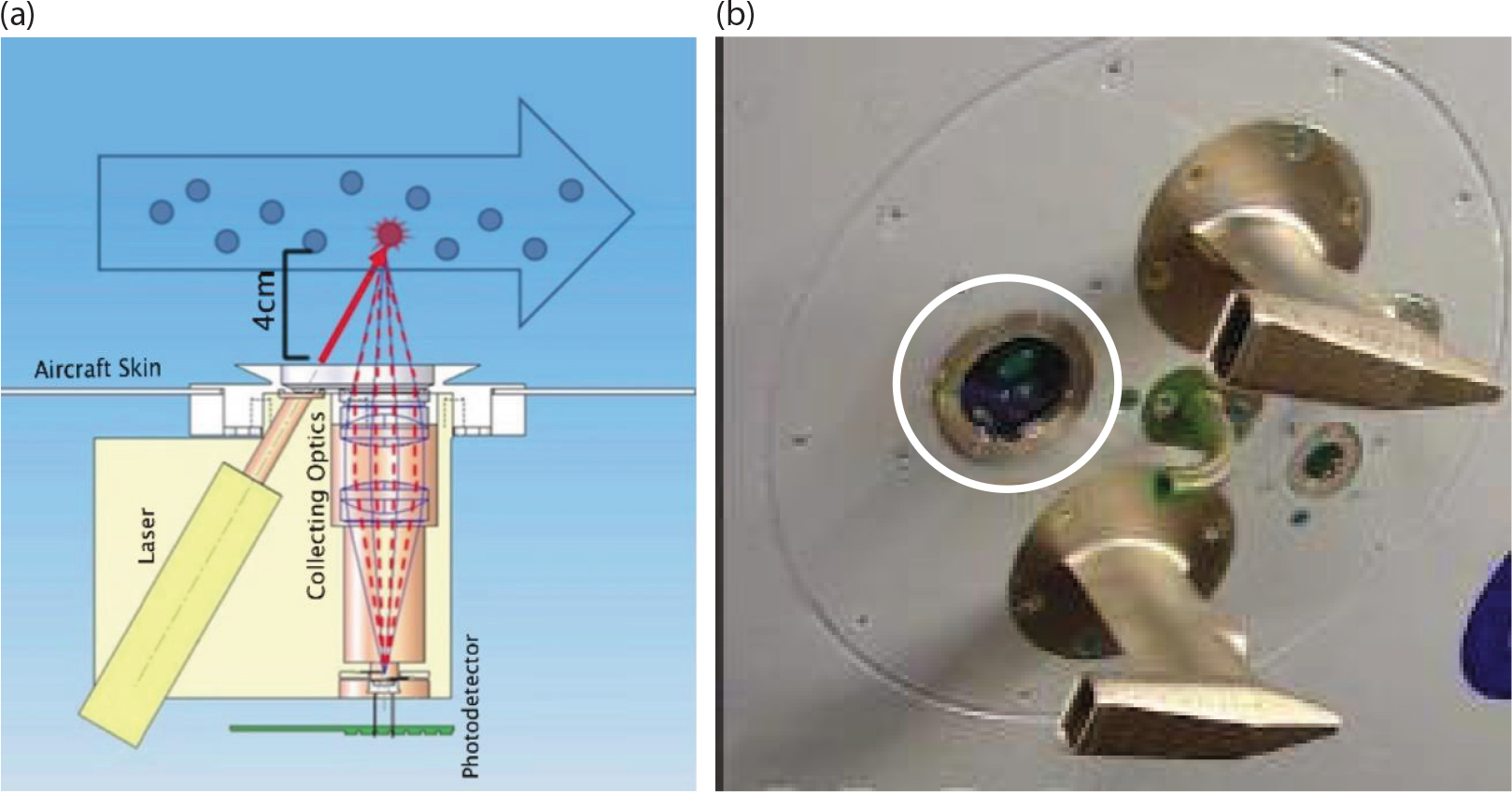
The BCP optical layout is shown in the schematic (a) illustrating the relative positioning of the laser, collection optics and the photodetector with respect to the BCP heated window that is mounted flush with the aircraft skin. The photograph (b) shows the BCP window, circled in white, on the aircraft mounting plate.
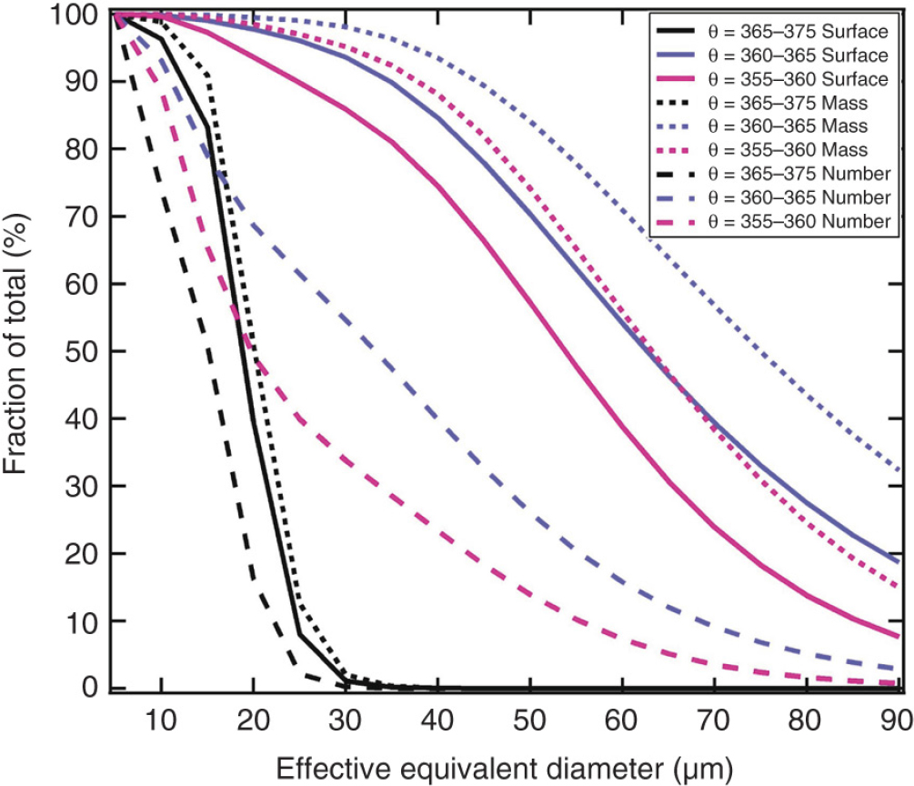
Fig. 2
The cumulative size distributions shown here are derived from the parameterised distributions from Frey et al. (2011), expressed as the percent of total number, surface and mass concentrations for the potential temperature ranges.
Table 1. General Statistics for the In-Service Aircraft Flights
D-AIGTJuly 2011941666223°S70°N−97°W138°E23 3245591 (24)3193 (14)14 540 (62)196 (2)China Airlines
B-18806June 2012147975179°S69°N−180°W180°E36 1946190 (17)3963 (11)26 041 (72)365 (3)Air Francea
F-GLZUJune 201357839925°N56°N−83°W15°E201135 (67)63 (31)3 (2)<1 (<0.01)Cathay Pacific
B-HLRAugust 20131139577038°S40°N39°E153°E14 1442287 (16)1479 (10)10 378 (74)98 (1)IBERIA
EC-GUQFebruary 2014262233635°S57°N−119°W0°E896326 (36)337 (36)233 (28)5 (<1)Totals439920 55774 75914 529 (19)9035 (12)51 195 (69)665 (1)
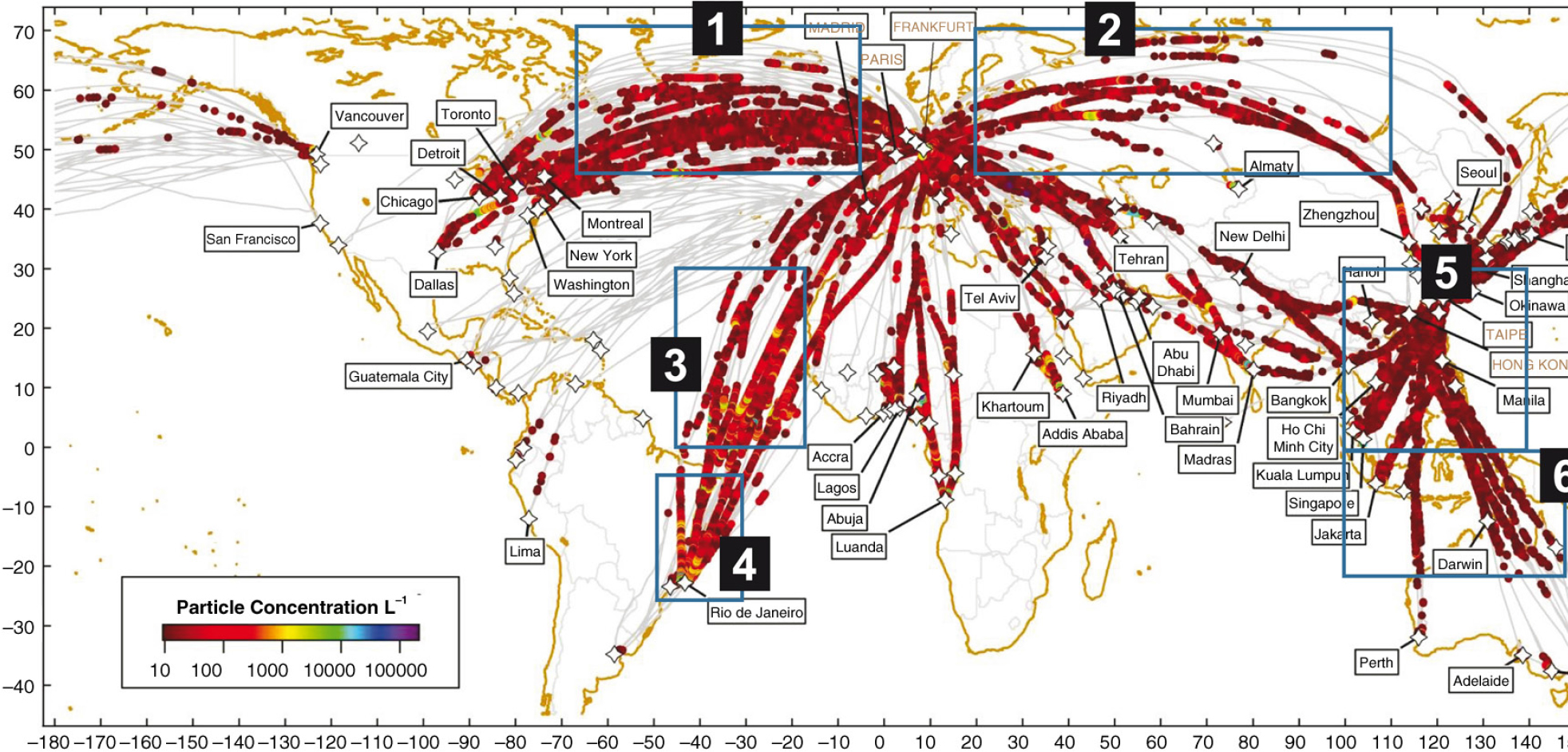
Fig. 3
This map lays out a summary of all the flight trajectories of the five aircraft from 2012 to 2014. The filled circles mark cloud encounters. The colour is proportional to the number concentration. The six numbered regions are (1) extratropical Atlantic, (2) extratropical Eurasia, (3) tropical Atlantic, (4) Eastern Brazil, (5) Southeast Asia maritime/continental and (6) New Guinea maritime/continental. The cloud properties in these regions are analysed and compared by season.
Table 2. Cloud size, altitude and temperature
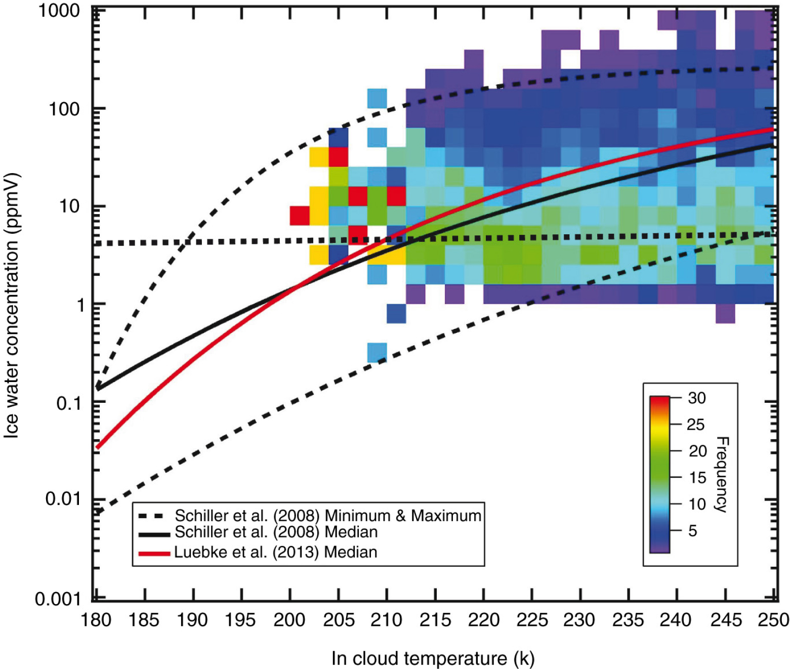
Fig. 4
The average derived ice water content (IWC) from 19 060 clouds is shown as a function of average cloud temperature. Each pixel represents the frequency with which the particular IWC–temperature pair occurred. The upper and lower black dashed and solid lines represent the minimum, maximum and median IWC as a function of temperature from the data set compiled by Schiller et al. (2008). The solid red line is the median value from Luebke et al. (2013). The black dotted line is the BCP median IWC.
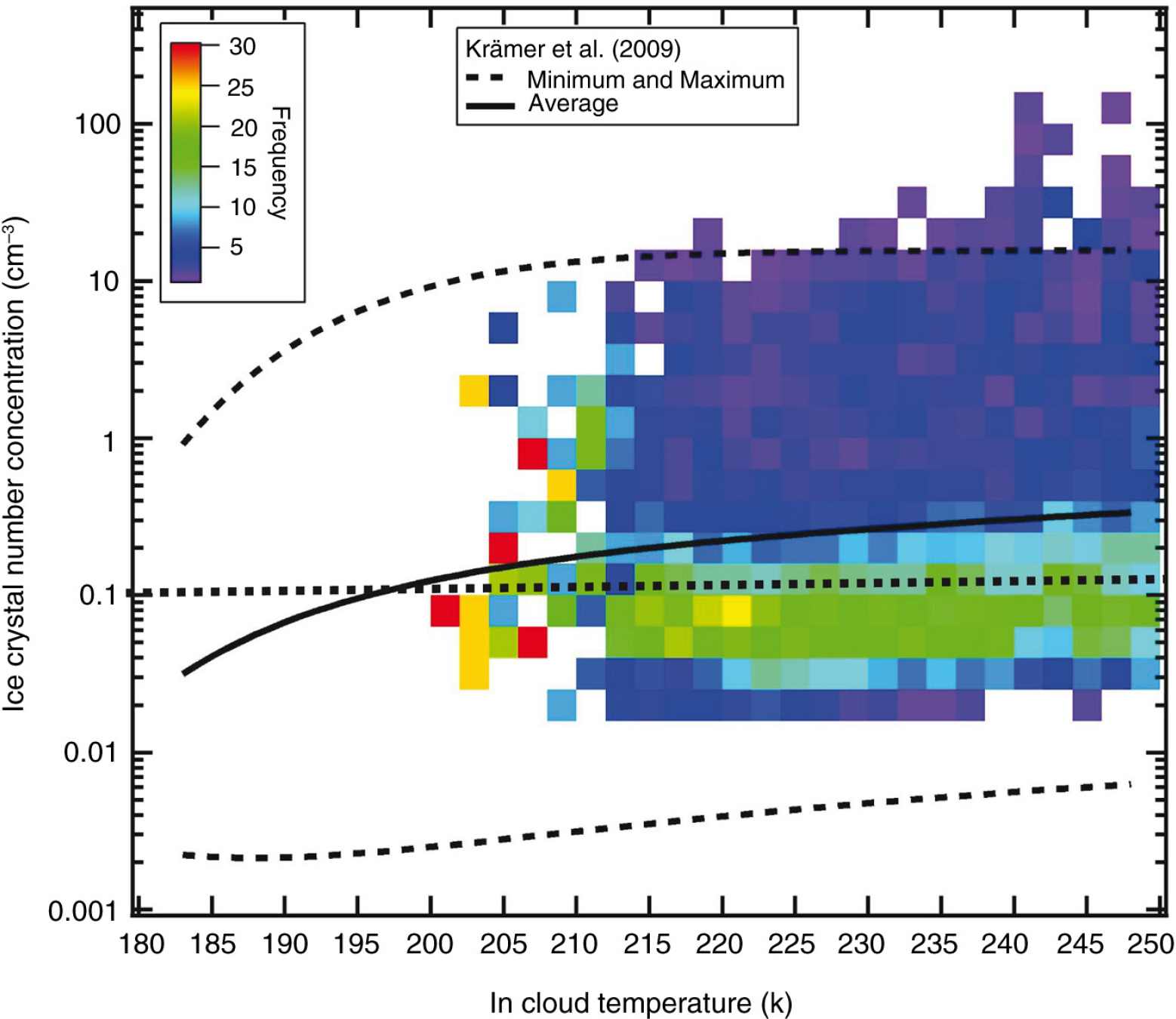
Fig. 5
This figure is the same as Fig. 4 except the average number concentration, N i, is shown as a function of temperature. The solid and dashed lines represent the median, minimum and maximum concentration as a function of temperature from the data set compiled by Krämer et al. (2009). The black dotted line is the BCP median N i.
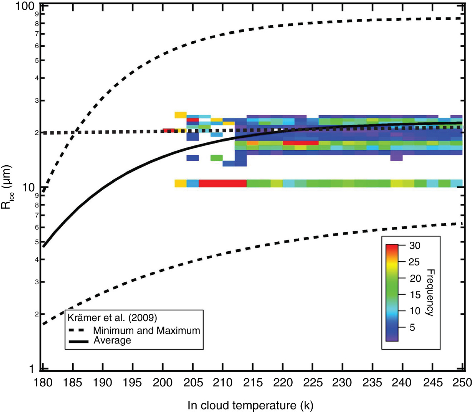
Fig. 6
This figure is the same as Fig. 4 except the average particle radius, R i, is shown as a function of temperature. The solid and dashed lines represent the median, minimum and maximum radii as a function of temperature from the data set compiled by Krämer et al. (2009). The black dotted line is the BCP median R i.
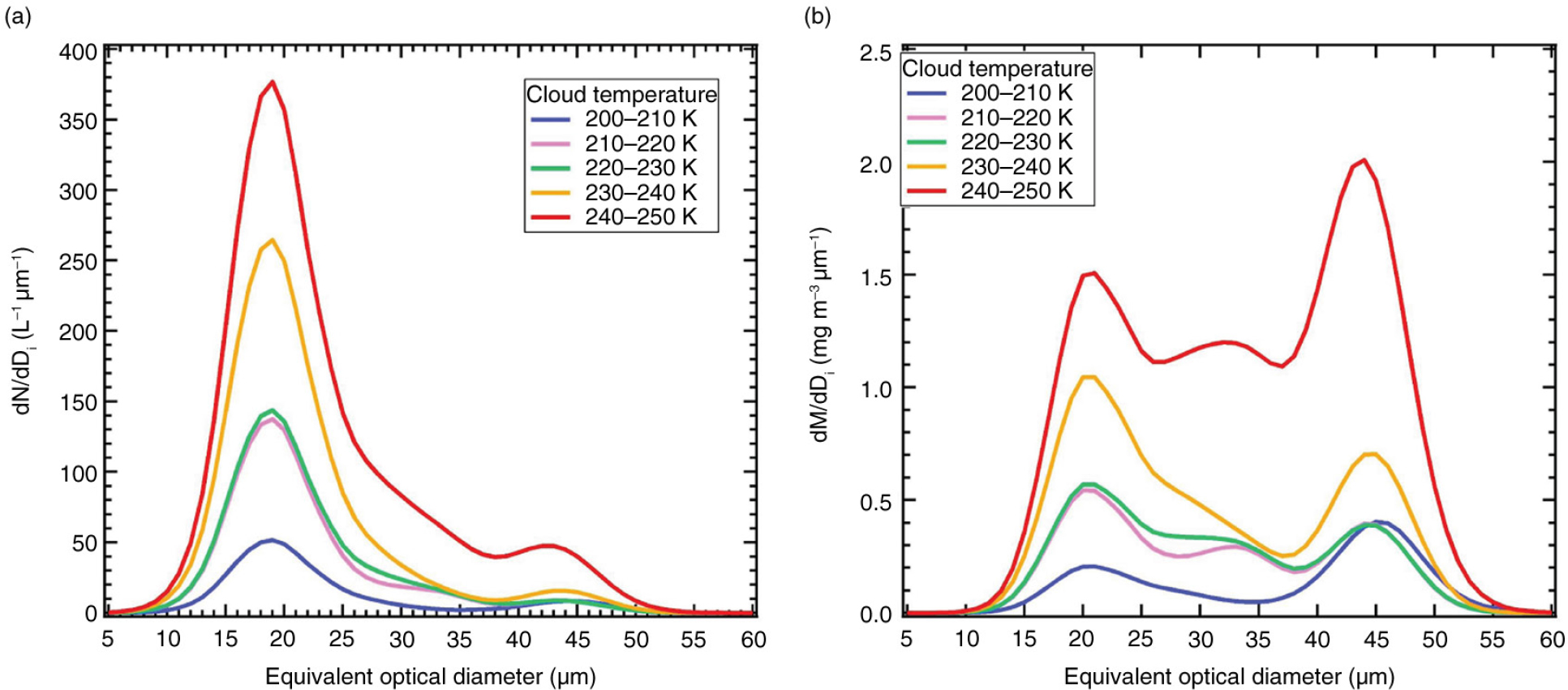
Fig. 7
This figure illustrates the (a) number and (b) mass size distributions as a function of five temperature ranges for the same cloud events used to construct Figs. (4–6).
Table 3. Cloud microphysical properties
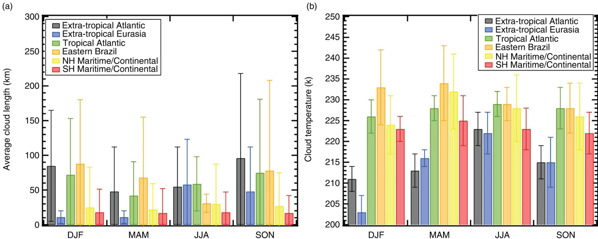
Fig. 8
The seasonal variation of (a) the average cloud size and (b) cloud temperature are summarised in this figure for the six regions. The vertical bars represent the standard deviations about the average.
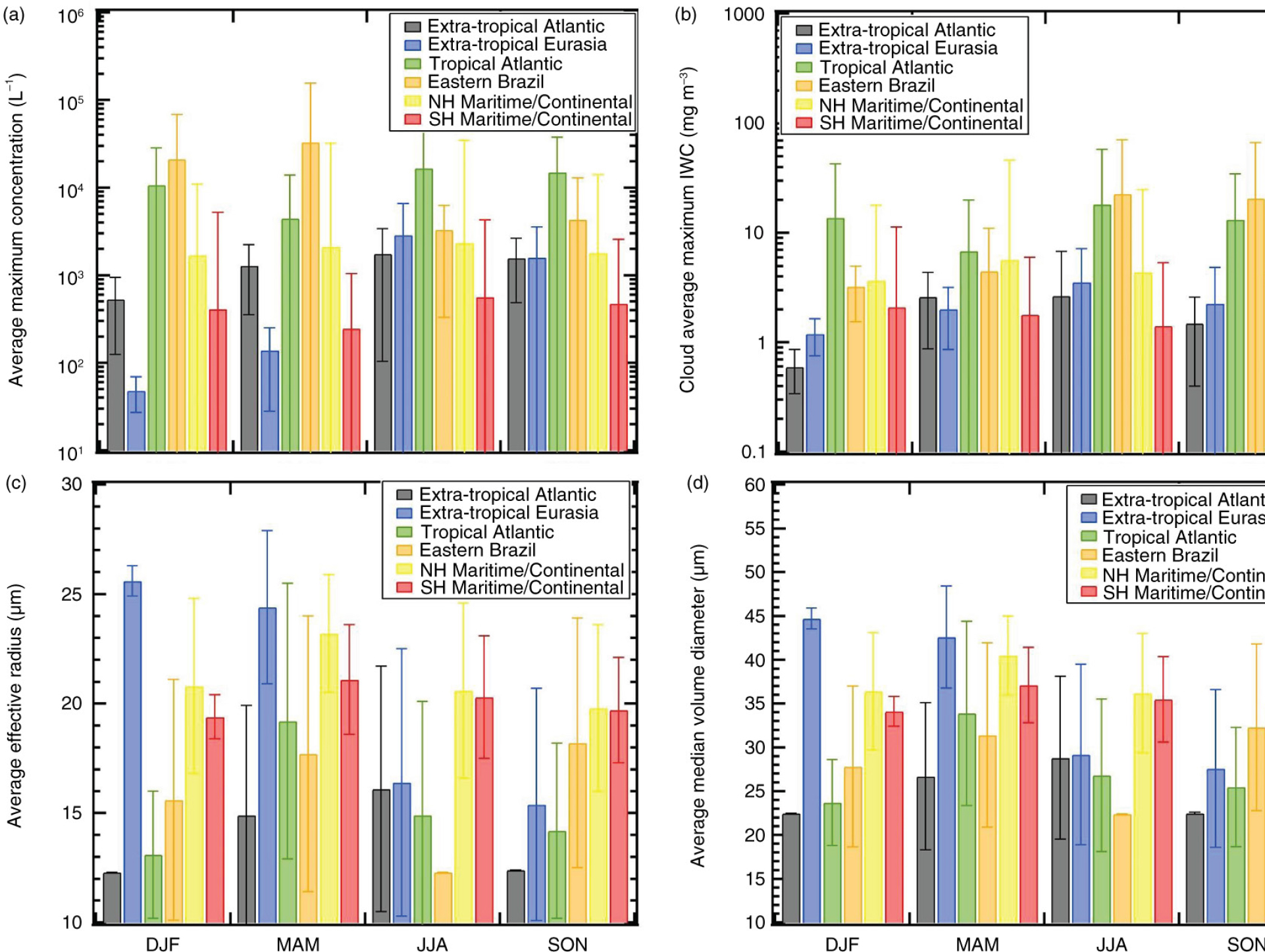
Fig. 9
This figure is similar to Fig. 8 but for the seasonal variations of the (a) average maximum number concentration (b) ice water concentration (c), effective radius and (d) median volume diameter.
Table 4. Microphysical Properties of Clouds by Region
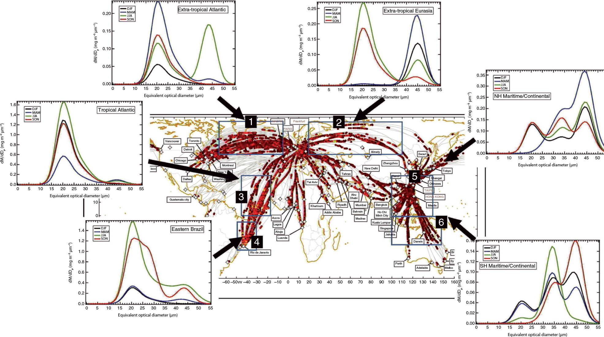
Fig. 10
The average size distributions of the mass concentrations are shown here for the six geographic regions measured over all cirrus clouds in December, January and February (black), March, April and May (blue), June, July and August (green) and September, October and November (red).
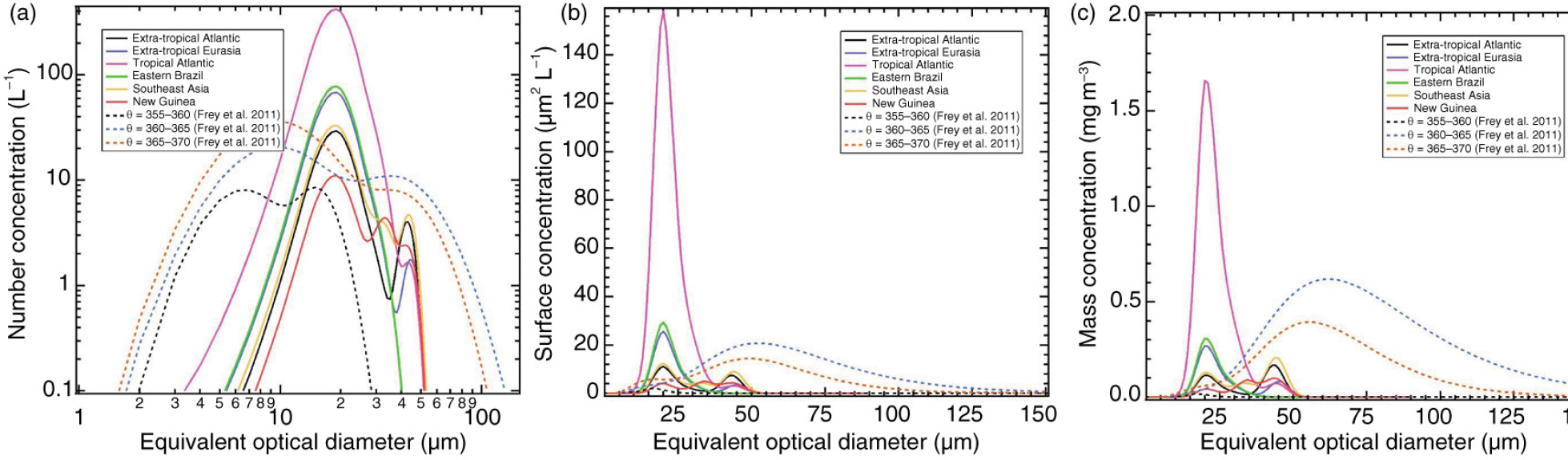
Fig. 11
The parameterised size distributions of (a) number, (b) surface and (c) ice water content, from Frey et al. (2011), are compared here with the regional spectra averaged over the summer flights.
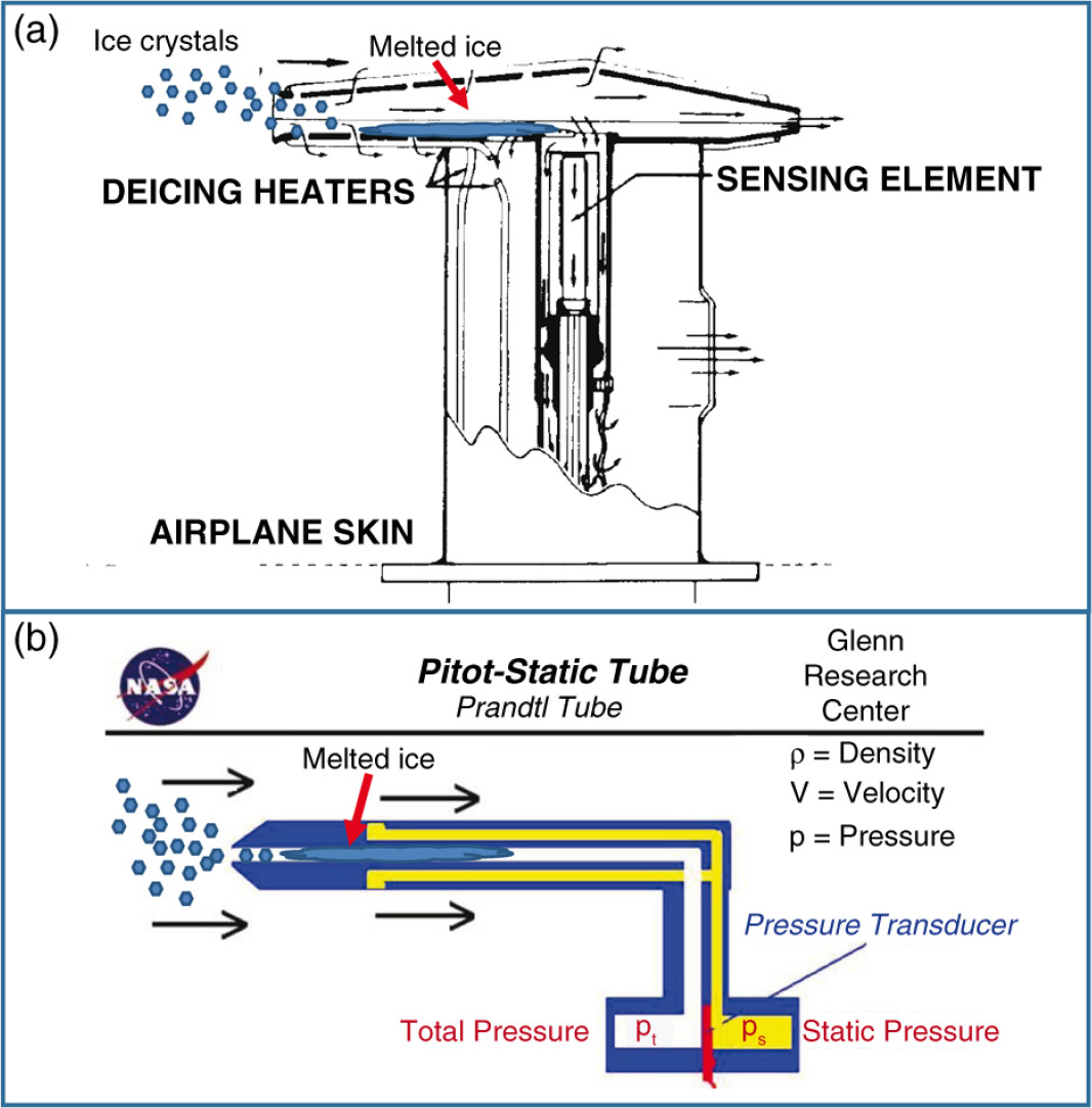
Fig. 12
As shown in these diagrams, (a) the aircraft temperature sensor and (b) airspeed sensor are susceptible to interference from high concentrations of ice crystals that enter the inlet and are melted by the sensor heaters, subsequently contributing to erroneous measurements.
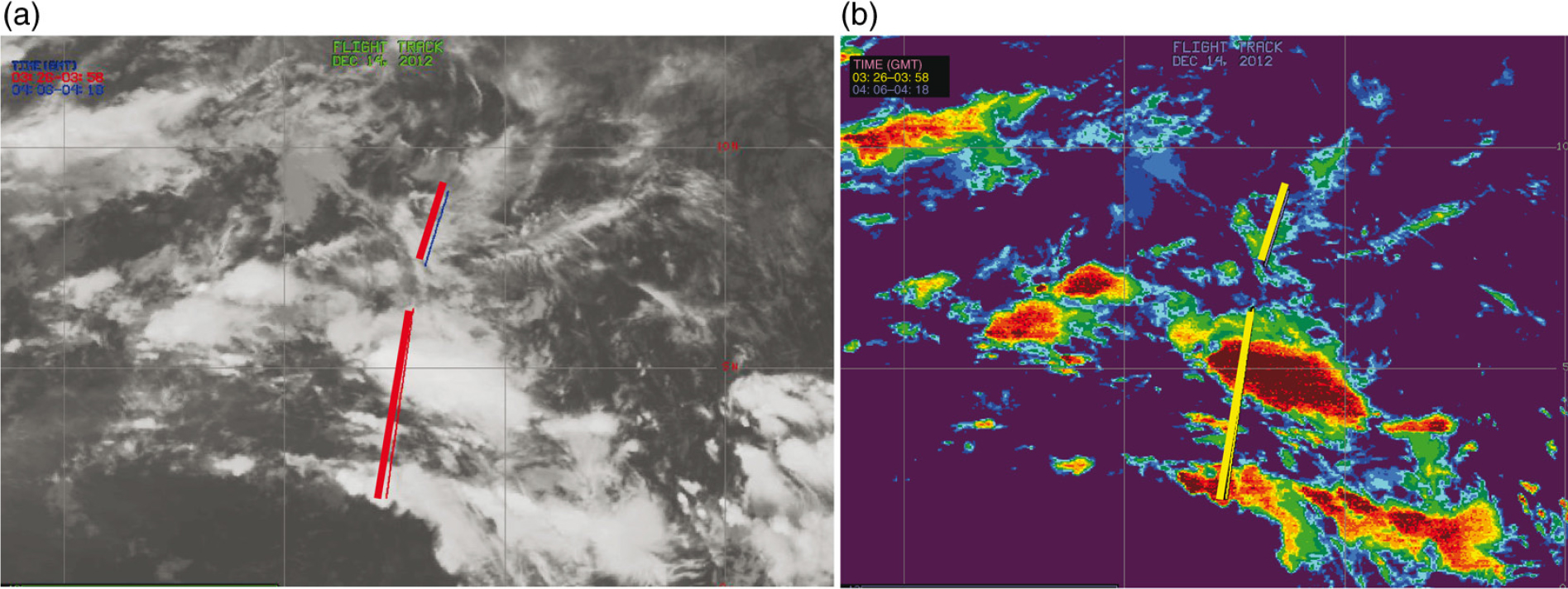
Fig. 13
The flight track of the aircraft through the clouds on December 14, 2012 is shown on the (a) visible and (b) brightness temperature difference (BTD) images from Meteosat-9. The BTD is the difference between the water vapour and infrared intensities.
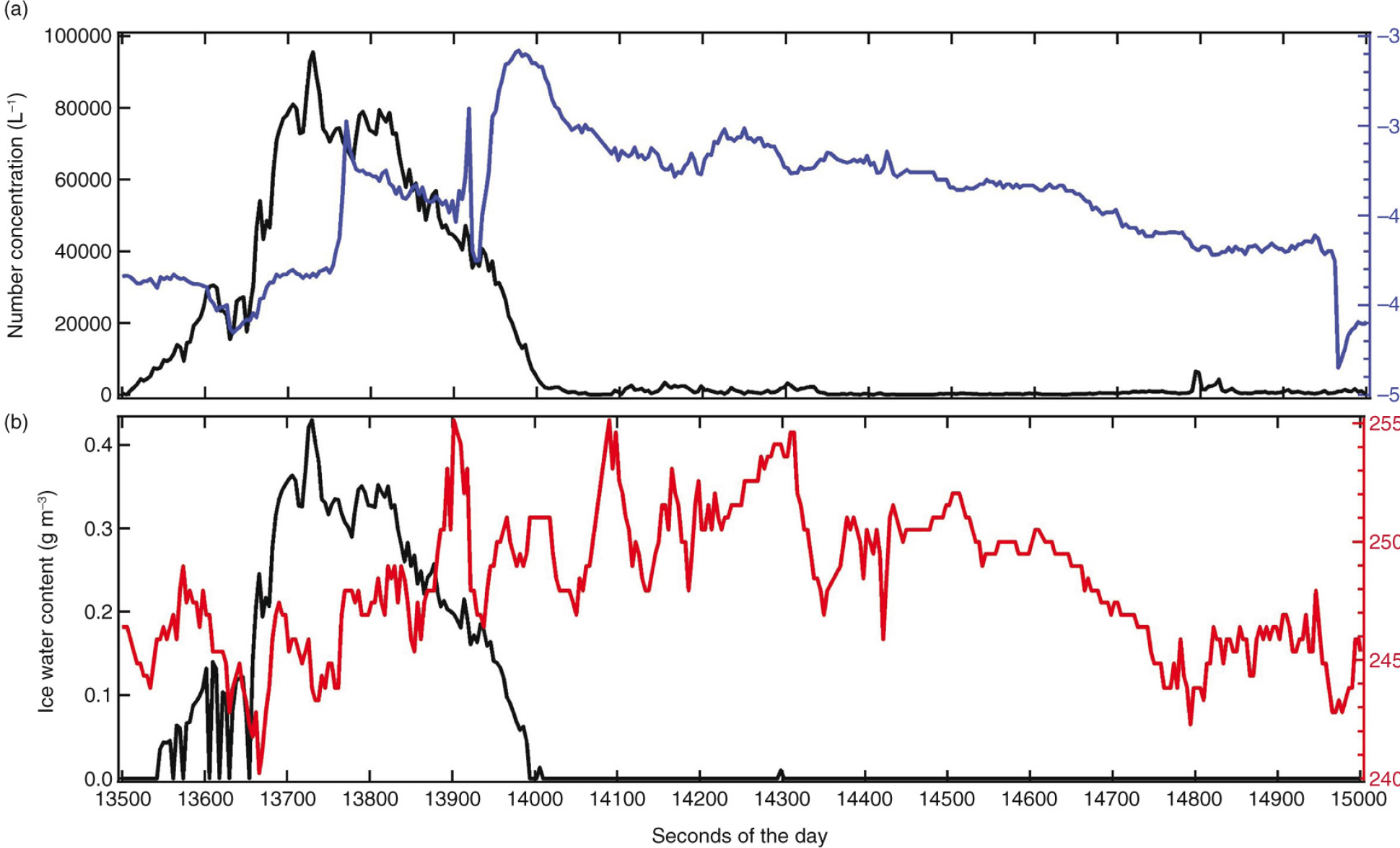
Fig. 14
Time series of (a) number concentration (black) and temperature (blue) and (b) ice water content (black) and airspeed (red).
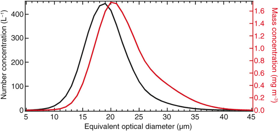
Fig. 15
This is the average size distribution of the number (black) and mass (red) concentrations during the high ice crystal event shown in Fig. 14.
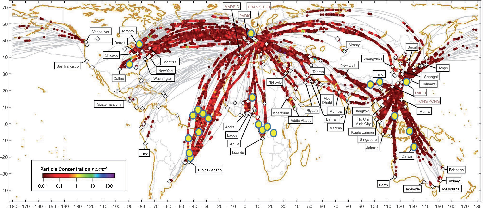
Fig. 16
There were 22 temperature anomalies recorded during the three years of measurements from 2012 to 2014. The yellow filled circles indicate temperature anomalies of greater than 5°C.