
1. Introduction
Cirrus clouds have been the subject of numerous airborne studies starting more than 60 yr ago when Weikmann (1947) collected ice crystals on oil-coated slides from the cockpit of his single engine aircraft flying over Germany. Twenty years later Braham and Spyers-Duran (1967) collected ice crystals with a replicator on their research aircraft, flying in clear air below cirrus clouds to document the precipitating cirrus that might seed lower clouds. Their measurements, made in the summer over Minnesota, USA, showed that cirrus crystals could survive falling long distances in dry air. In their study, a majority of the crystals were columnar with an average length of about 40 µm. In the early 1970s, measurements were made in cirrus with the National Center for Atmospheric Research (NCAR) Sabreliner and the University of Chicago Lodestar (Heymsfield and Knollenberg, 1972; Heymsfield, 1975) using the newly developed optical array probe (Knollenberg, 1970) that allowed a much larger and continuous sample of crystals to be taken. A formvar replicator was also employed enabling the measurements to cover the size range from 10 µm to greater than 2000 µm. Those measurements, made during the summer over Colorado, Wyoming and Minnesota, showed that the largest size of crystals was between 10 and 30 µm with concentrations as high as 1000 L−1.
In 1980, Knollenberg et al. (1982) flew an optical array probe and a new single particle light scattering probe (Knollenberg, 1976) with a size range from approximately 2 to 50 µm on the NASA U-2 high-altitude aircraft over Panama, the first airborne cirrus measurements to be made in the tropics. All of the measurements were made in anvil cirrus with the highest number concentrations in the size range 10 and 50 µm, but the mass was mostly in crystals between 40 and 50 µm.
In the mid-1980s, a new research project to study stratus and cirrus clouds was initiated, the First ISCCP Regional Experiment (FIRE), in support of the International Satellite Cloud Climatology Project (ISCCP). The FIRE objective to study the role of clouds in climate was addressed using the NCAR Sabreliner to conduct cirrus measurements over the US Midwest (Cox et al., 1987; Heymsfield et al., 1990). The results from these and earlier studies are summarised by Dowling and Radke (1990).
In August 1986, measurements were made in clouds over Darwin, Australia with the NASA ER-2 as part of the Stratospheric–Tropospheric Exchange Project (STEP). The Forward Scattering Spectrometer Probe (FSSP) with a size range of 2–50 µm (Knollenberg, 1976) was deployed to measure cirrus clouds. During these flights, ice crystal concentrations in excess of 100 000 L−1 were measured at altitudes between 12 and 13 km and temperatures from −55°C to −60°C. The highest concentrations were found for crystal sizes between 10 and 30 µm (Knollenberg et al., 1993).
A number of other cirrus studies were conducted during the 1990s, including the Central Equatorial Pacific Experiment (CEPEX) that looked at the extensive cirrus that formed over warm maritime areas during March and April of 1993 (Heymsfield and McFarquhar, 1996; McFarquhar and Heymsfield, 1996, 1997). This was followed by the Subsonic Aircraft: Contrails and Cloud Effects Special Study (SUCCESS) that used multiple aircraft to target contrails and cirrus (Lawson et al., 1998a).
Beginning in the late 1990s and continuing into the present, there have been many other aircraft programmes that measured the microphysical properties of cloud in the tropics, mid-latitudes and the Arctic, for example, Gayet et al. (2004, 2006, 2011), Schiller et al. (2008), Krämer et al. (2009) and Luebke et al. (2013), de Reus et al. (2009), Jensen et al. (2010), Frey et al. (2011), and the many references included with these studies that describe more than 20 field programmes that targeted diverse regions of the world.
All of these field programmes had three things in common: most of them were of short duration, lasting at most 1–2 months; most of them were conducted during the summer or autumn; and none of them measured cirrus clouds over the same region during different seasons. There is great value in what has come out of all of these past field projects. We now know much more about the microphysical properties of cirrus clouds that are generated by outflow from deep convection, lifting by cold fronts or vertical motion caused by gravity waves. Extensive comparisons have been made between in situ measured microphysical properties and those derived from satellite images. Models have been developed that can simulate cirrus development under different conditions. However, a question remains: Do the cirrus that have been measured represent cirrus on a global scale? In general, the strategy for cloud sampling during an intensive field campaign is to target the most visually thick regions of the cloud. Hence, although this will likely measure the regions of highest concentrations, with results that are useful for a better understanding of cloud microphysics, the results from these campaigns may not be statistically representative of cirrus properties worldwide. This is an important consideration when studying the climate impact of cirrus.
One of the driving factors behind the development of the European Research Infrastructure programme IAGOS (In-service Aircraft for a Global Observing System) was the desire to build a database of global measurements, over an extended time period, in order to create a source of information that would be truly representative across all temporal and spatial scales (Petzold et al., 2015). The backscatter cloud probe (BCP) is part of the IAGOS package that has now been flying on Airbus 330/340 commercial aircraft since September, 2011. In the following study, we describe this instrument, its uncertainties and limitations and the cloud microphysical properties that are derived from the measurements. The results are a compilation of 3 years of data presented in tabular and graphical form to allow the reader to understand the wealth of information that is available for future evaluations of the impacts of clouds on climate and the underlying physics that lead to the formation and evolution on local, regional and global scales.
2. Data collection methodology
2.1. Ice crystal measurement technique
The cloud data were collected using the BCP whose operating principles and measurement limitations are described in detail by Beswick et al. (2014). The BCP, shown schematically in Fig. 1a, is an optical spectrometer that detects the light scattered in a backward cone by individual atmospheric particles that pass through the centre of focus of a 650-nm wavelength laser beam generated by a diode. The collected photons are converted to an electrical current by a photodiode and the peak current is analysed to provide an equivalent optical diameter (EOD). In the application described here, that is, measurements from a commercial airliner, the BCP microprocessor uses the derived EOD to select one of 10 size bins in the interval from 5 to 75 µm, and increments a 10-channel frequency histogram that accumulates every 4 seconds. At the end of each 4-second sampling period, the number of particle events recorded in each of the 10 channels is transmitted serially to the data system, which stores this information along with various voltages and temperatures that are used to assess the data quality and health of the system.
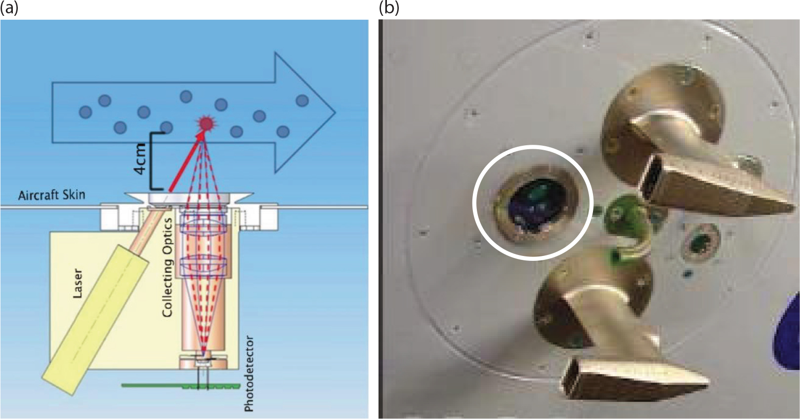
Fig. 1
The BCP optical layout is shown in the schematic (a) illustrating the relative positioning of the laser, collection optics and the photodetector with respect to the BCP heated window that is mounted flush with the aircraft skin. The photograph (b) shows the BCP window, circled in white, on the aircraft mounting plate.
The recorded frequency histograms are evaluated during post-processing to provide size distributions of number and mass concentration as a function of the EOD. This processing involves an inversion technique that takes into account the intensity distribution of the laser beam and the inherent ambiguities that are related to the scattering cross-section as a function of particle diameter (Beswick et al., 2014). The inversion allows the derivation of a size distribution that not only has more channels than the original data, but also extends to larger EODs due to the nature of the undersizing of some fraction of particles passing through less intense regions of the laser beam.
For the current study, in addition to the number and mass size distributions, the bulk parameters number concentration (L−1), ice water content (mg g−3), effective radius (µm), mass weighted volume diameter (µm) and extinction coefficient (km−1) are derived from the number size distribution
where n i is the number of counts in channel i, c i is the concentration per size interval, SV is the sample volume calculated from the product of the BCP sample area and the aircraft airspeed, ρ is the crystal density and d i is the crystal EOD. In the studies reported here, the ice crystals are assumed spherical with an ice density of 0.5 g cm−3. The definition of R eff is taken from Fu (1996) for cirrus clouds.
2.2. Measurement limitations and uncertainties
The EOD used in our evaluations is by definition the size of a water droplet with refractive index 1.33−0.0i (at 650 nm wavelength) that would have produced the intensity of scattered light that was measured from the detected ice crystal. This definition is used in order to apply the Mie scattering theory (Mie, 1908) to the measured light intensity and derive a crystal parameter that we will use as an operational definition of size from which all of the bulk parameters are calculated. This definition introduces an uncertainty into the derived bulk parameters whose calculations include different moments of the size distribution, that is, B ext~d 2 and IWC~d 3. The uncertainties in deriving d i and c i are approximately ±20% (Beswick et al., 2014) for water droplets, but for aspherical ice crystals the uncertainty in d i may be more than ±50%, depending on the average aspect ratio of the crystal. In addition, without knowing the actual shape or habit of the ice crystals that are detected by the BCP, the ice density ρ in cirrus could vary from 0.2 to 0.9 g cm−3 (Dowling and Radke, 1990). Selecting an average density of 0.5 in the calculations limits the uncertainty to a maximum of 100% in ice density. Hence, the root mean square errors (RSS) in B ext, IWC, R eff and MVD are approximately ±70%, ±180%, ±50%, ±50%, respectively, for ice crystals.
An additional source of uncertainty that can cause over-counting by the BCP, as well as mis-sizing, is the shattering of large ice crystals on the fuselage of the aircraft upstream of the BCP sample volume (Beswick et al., 2014). There have been no observational studies to assess the magnitude of this effect; however, one modelling evaluation (Engblom and Ross, 2003) demonstrated with simulations that ice crystals hitting the leading edge of aircraft wings can bounce, even as they shatter, quite some distance from the aircraft skin. Hence, we can only speculate at the moment that ice crystal shattering may lead to potentially high biases in the derived number concentrations and IWC. As discussed further in Section 4, these artefacts may also have a real impact on other aircraft sensors.
Another issue related to the impact on particle measurements due to airflow around the aircraft fuselage is that of shadow and enhancement zones (King, 1984a, 1984b; Norment 1985, 1988; Twohy and Rogers, 1993). Shadow zones are inside the boundary layer of air near the skin of the aircraft where particles cannot enter due to being carried by the streamlines. This was addressed by Beswick et al. (2014) for the BCP, who argued that the measurement results from comparison of the BCP with other instruments on two research aircraft, and the physically reasonable size distributions detected on the commercial aircraft, indicate that the sample area of the BCP is not in a shadow zone. Enhancement zones are regions of compressed airflow where inertial sorting of particles occurs due to velocity gradients. This is a potential source of measurement bias that cannot be ruled out until measurements like those done by Twohy and Rogers (1993) or modelling like King (1984a) and Norment (1985, 1988) are carried out. The general effect is to enhance the number concentration of some sizes while decreasing the concentration of others.
The BCP, as configured, has an upper EOD limit of 75 µm that is extended to 90 µm after applying the inversion algorithm. This upper threshold suggests that the bulk quantities that are derived from the size threshold, for example, N, IWC and B ext may be underestimated, possibly complicating the interpretation of the measurements. An exhaustive search of airborne studies of cirrus clouds was conducted on the literature over the past 10 yr. All of the papers that showed size distributions have been discussed in the Introduction section. The two that provide the basis for estimating how much number, surface area (extinction) or mass (IWC) might be beyond the size range of the BCP are by de Reus et al. (2009) and Frey et al. (2011). Both studies were focused on cirrus using instruments that, with overlapping size measurements, could detect ice particles from 2 µm to greater than 1000 µm. The measurements of de Reus et al. (2009) were made in the overshooting anvils of the ‘Hector’ clouds in Australia and those of Frey et al. (2011) in the anvils of deep convection clouds formed during the African monsoon. Both studies parameterised their size distribution as a function of potential temperature using multi-lognormal functions.
Although the results from these two studies are certainly not exhaustive, and only represent clouds in two regions over a short time period, they offer the means to estimate what fraction of the total number, surface area and mass was in crystals larger than the BCP size threshold for two projects. The cumulative distributions shown in Fig. 2 were generated by integrating the lognormal function using the parameters given in Table 2 of Frey et al. (2011) for three potential temperature ranges that are the same as the majority of the BCP measurement in our study. The measurements from the BCP in this study were made more than 90% of the time in the potential temperature range from 355°C to 365°C. From this figure, we observe that the maximum number, surface area and mass beyond 90 µm, in this temperature range, are ≅0%, 20 and 30% of the totals, respectively.
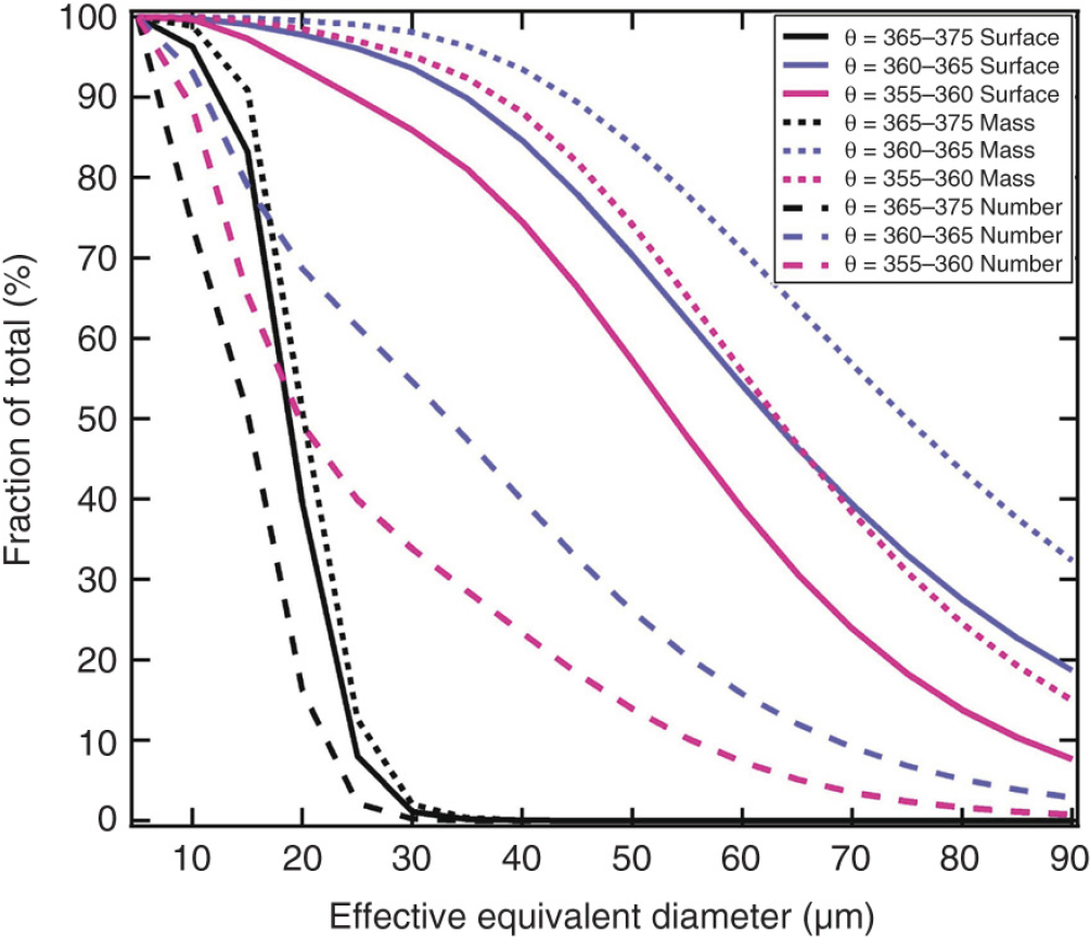
Fig. 2
The cumulative size distributions shown here are derived from the parameterised distributions from Frey et al. (2011), expressed as the percent of total number, surface and mass concentrations for the potential temperature ranges.
Another method in which the presence of large particles can be identified from the BCP measurements is to evaluate how many size spectra were measured when there were counts in the last channel of the size histogram. This would indicate that there might be larger particles that had passed through the beam but whose signal saturated the detectors. In the potential temperature range from 355°C to 365°C the size distributions had counts in the last channel 12% of the time. Hence, although it is important to measure the whole range of crystal sizes if possible, we assess that there is an underestimate of approximately 20% of the surface and 30% of the mass less than 15% of the time.
2.3. Data collection from IAGOS platforms
The BCP is part of the core measurement package installed as part of the IAGOS programme (Petzold et al., 2015) on five Airbus 330/340 aircraft (as of January 2015). Figure 1b is a photo of one of the mounting plates that hold the inlets for the gas phase measurements and the window (circled in white) behind which the BCP is mounted. Table 1 lists the five aircraft that are currently carrying the BCP and the dates when the BCP was first put into operation. This table also summarises the number of flights with the BCP that have been made up to the end of 2014, the total number of flight hours and the geographic range over which clouds have been sampled.
Table 1. General Statistics for the In-Service Aircraft Flights
D-AIGTJuly 2011941666223°S70°N−97°W138°E23 3245591 (24)3193 (14)14 540 (62)196 (2)China Airlines
B-18806June 2012147975179°S69°N−180°W180°E36 1946190 (17)3963 (11)26 041 (72)365 (3)Air Francea
F-GLZUJune 201357839925°N56°N−83°W15°E201135 (67)63 (31)3 (2)<1 (<0.01)Cathay Pacific
B-HLRAugust 20131139577038°S40°N39°E153°E14 1442287 (16)1479 (10)10 378 (74)98 (1)IBERIA
EC-GUQFebruary 2014262233635°S57°N−119°W0°E896326 (36)337 (36)233 (28)5 (<1)Totals439920 55774 75914 529 (19)9035 (12)51 195 (69)665 (1)
In Table 1, there are also several columns summarising the cloud sampling statistics for each aircraft and for the programme as a whole. In this study, there are two cloud detection threshold levels used in the compilation of cloud statistics and description of the cloud properties. The first threshold that defines a cloud event is when the measured concentration is greater than 50 L−1. This corresponds to a detection of approximately 13 particles within the BCP 4-second sampling period at an average cruise speed of 250 m s−1 for commercial airliners. Assuming Poisson statistics for estimating the counting uncertainty, this corresponds to a sampling error of ±25%. Cirrus clouds have crystal concentrations that range from several per litre to thousands per litre (Mace et al., 2001; Krämer et al., 2009); hence, selecting a threshold value of 50 L−1 falls below the concentrations observed in previously sampled cirrus (Krämer et al., 2009) while maintaining the sampling uncertainty at a reasonable value.
The second cloud threshold used in the analysis is the requirement that at least four adjacent channels in the size distribution are non-zero. This requirement is needed in order for the inversion to produce a reasonable, unambiguous size distribution from the measured spectrum (Beswick et al., 2014). Hence, in the discussions on cirrus microphysical properties, all of the derived bulk properties are calculated from the inversion extracted size distributions after satisfying the four-channel threshold.
As observed in Table 1, the Lufthansa, China Air and Cathay Pacific aircraft sampled the largest number of clouds: 23 000, 36 000 and 14 000, respectively. Taking into account the total number of flight hours, these three aircraft also spent the highest percentage of time in clouds, that is, 2, 3 and 1%. The five aircraft sampled a total of 74 759 clouds between 2012 and 2014 for a total of 664 accumulated hours in cloud.
The three aircraft that sampled the most clouds are those whose flight routes take them over the Inter-Tropical Convergence Zone (ITCZ), where the outflow from deep convection produces large areas of high-level clouds. This is underscored by the percentage of the clouds that were encountered by these aircraft above 8000 m. All three sampled more than 60% of the clouds above this altitude.
Although the focus of the current study is cirrus, Table 1 also lists the number of clouds that were sampled during take-off and landing (low and mid-level). These are an interesting subset of the BCP measurements that contain useful information on the vertical structure of more than 23 000 clouds that are currently being analysed.
3. Cirrus properties
Figure 3 illustrates the flight trajectories of the IAGOS fleet from 2012 to 2014, with colour-coded markers that indicate where clouds were encountered and the number concentration. The numbered boxes delineate regions that are discussed below: (1) extratropical Atlantic, (2) extratropical Eurasia, (3) tropical Atlantic, (4) Eastern Brazil, as well as the maritime continent that has been divided in (5) Southeast Asia and (6) New Guinea. The sixth region covers more than just New Guinea but the nomenclature is used here as a convenience to describe that whole region. These are regions where clouds were frequently encountered, clouds that climatologically are formed as a result of deep convection, gravity waves or other synoptic scale vertical motions.
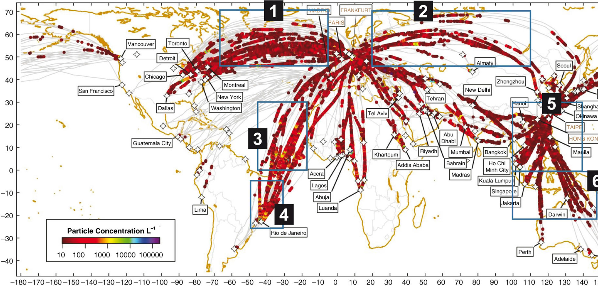
Fig. 3
This map lays out a summary of all the flight trajectories of the five aircraft from 2012 to 2014. The filled circles mark cloud encounters. The colour is proportional to the number concentration. The six numbered regions are (1) extratropical Atlantic, (2) extratropical Eurasia, (3) tropical Atlantic, (4) Eastern Brazil, (5) Southeast Asia maritime/continental and (6) New Guinea maritime/continental. The cloud properties in these regions are analysed and compared by season.
The data are further parsed according to the four seasons: (1) NH winter (SH summer) – December, January and February (DJF), (2) NH spring (SH fall) – March, April and May (MAM), (3) NH summer (SH winter) – June, July and August (JJA) and (4) NH fall (SH spring) – September, October and November (SON). Additional parsing of the data is done depending on the cloud's extinction coefficient derived from the measurements [eq. (3)]: (1) subvisible cirrus (SVC) when B ext<0.1 km−1, (2) thin cirrus when 0.1≤B ext<1.0 and (3) opaque cirrus for B ext≥1.0. The cirrus categories of SVC, thin and opaque are used by the remote sensing community based on definitions put forth by Sassen and Cho (1992) to describe the vertical thickness of the cloud; however, since commercial aircraft normally fly a straight and level course we use a modified definition based on the in situ, horizontal path measurements.
3.1. Cirrus seasonal statistics: size and temperature
The aircraft spent more than twice as much time in cloud (496 hours, 3.1%) during the summer and fall (S–F) months, than during the winter and spring (W–S) seasons (169 hours, 1.6%), as shown in the summary statistics in Table 3. The majority of clouds (6473) were encountered during the summer months, followed by 3384 in the fall, 1258 in the spring and 1064 in the winter. The relative frequency of occurrence, 53%, 28%, 10% and 9% (yellow highlighted numbers in Table 2), over these four seasons, does not vary with cloud optical thickness. Cirrus are formed from vertical motions driven by gravity waves, orographic barriers, frontal lifting or deep convection. The seasonal frequency in cloud encounters can be linked to deep convection in the summer and early fall, especially in the sub-tropical and tropical regions, although mid-latitudes also have a higher frequency of deep convection during these seasons. The distribution of cloud by opacity, however, shows no seasonal differences. Over the four seasons, the types most frequently sampled were thin (66–72%), followed by opaque (20–26%) and SVC (7–8%) clouds.
Table 2. Cloud size, altitude and temperature
The median and 75% quantile (third quartile) statistics are used in Table 2 to compare the size and temperature of the three cirrus types over the four seasons. The cloud size is expressed here as the cloud length calculated from the product of the time in cloud and the airspeed. The medians and third quartiles are used instead of the average and standard deviation since the frequency distributions of the cloud properties are positively skewed; hence, the average and standard deviation are biased by outliers in the tail of the distributions.
Regardless of the time of year, the cloud size is related to cirrus type with median cloud lengths of 13, 25 and 40 km and third quartile sizes of 9, 25 and 88 km, respectively for SVC, thin and opaque clouds. Regardless of the cirrus type, the winter, summer and fall seasons have approximately the same median and third quartile whereas the cloud size in the spring is smaller. This difference is particularly notable for the opaque clouds where the median and third quartile sizes in the springtime are 30 and 69 km in length compared to an average median and third quartile of 43 and 94 km for the other three seasons. The anomalous decrease in cloud size during springtime is puzzling as it extends over all cloud types giving no clue as to the source of the difference. A more in-depth analysis of the seasonal synoptic and mesoscale meteorology is needed to provide a better understanding of this phenomenon.
A cautionary note is that the cloud lengths presented here may not be representative measures of the cloud's horizontal or vertical size. Although a relatively large number of cirrus were sampled, in the absence of complementary measurements (e.g. satellite images), the values presented here are useful primarily to compare the relative sizes of cloud types. In addition, these values can be considered a truly random sampling of clouds since commercial aircraft follow pre-programmed routes that will normally not deviate unless severe weather is encountered. Therefore, the cloud measurements obtained from commercial aircraft constitute a sample obtained strictly by chance. This sampling is very different from the ones carried out during research projects when aircraft intentionally fly through selected clouds and usually through their thickest regions.
An examination of cirrus temperature shows that SVC clouds are the coldest over all seasons, with an average median of −45.3°C, increasing to −42.1°C and −36.9°C for the thin and opaque clouds, respectively. The median and third quartile cirrus temperatures decrease from a springtime maximum to a minimum in the winter. The seasonal temperature range is relatively small for the SVC which has minimum and maximum third quartile temperatures of −47.5 and −43.2, respectively. For the thin and opaque clouds the range is larger, −45.7 to −37.9 and −40.9 to −32.4, respectively. The transition in temperature from spring to summer to fall is gradual, only decreasing by two or three degrees between seasons, whereas the temperature increase from winter to spring is much larger, eight degrees for both thin and opaque clouds.
3.2. Cirrus microphysical properties
Figures (4–6) present a compilation of the average IWC, number concentration (N i ) and ice crystal radius (R i ) as a function of average cloud temperature. We present our results in the format introduced by Schiller et al. (2008) and subsequently followed by Krämer et al. (2009) and Luebke et al. (2013). This allows direct comparison of the measurements from the BCP with those that were made with other instruments mounted on research aircraft that were deployed during more than two dozen field campaigns throughout the years. Also, to correspond to the units used for IWC in these three publications, g m−3 has been converted to ppmV using the air density.
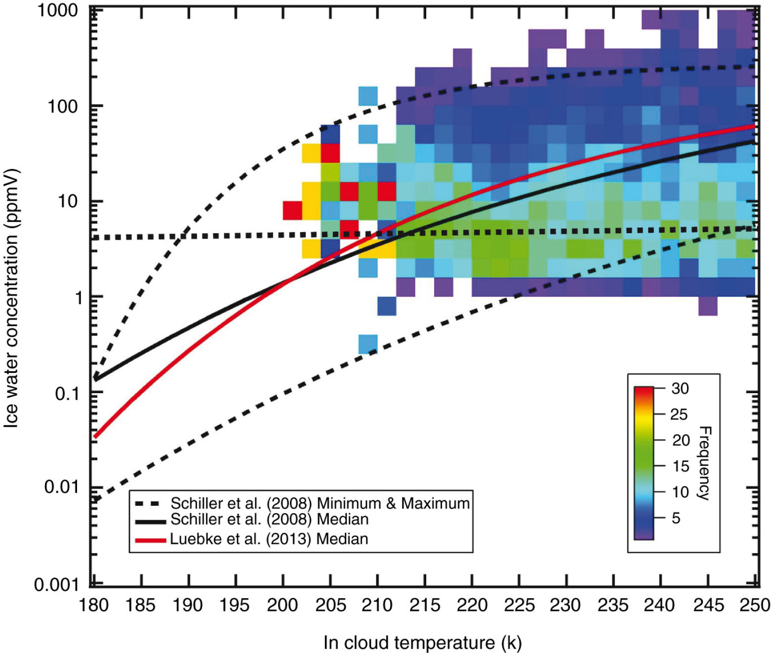
Fig. 4
The average derived ice water content (IWC) from 19 060 clouds is shown as a function of average cloud temperature. Each pixel represents the frequency with which the particular IWC–temperature pair occurred. The upper and lower black dashed and solid lines represent the minimum, maximum and median IWC as a function of temperature from the data set compiled by Schiller et al. (2008). The solid red line is the median value from Luebke et al. (2013). The black dotted line is the BCP median IWC.
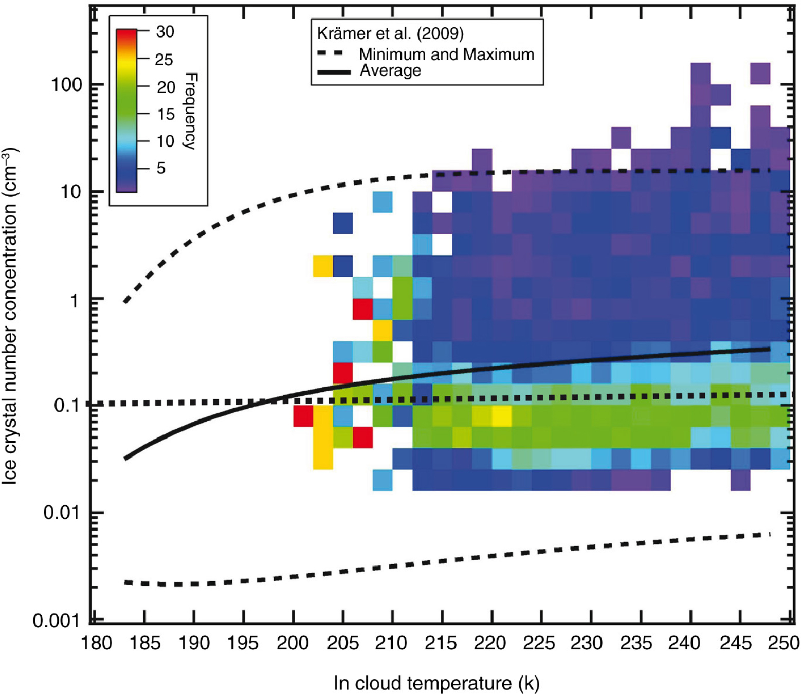
Fig. 5
This figure is the same as Fig. 4 except the average number concentration, N i, is shown as a function of temperature. The solid and dashed lines represent the median, minimum and maximum concentration as a function of temperature from the data set compiled by Krämer et al. (2009). The black dotted line is the BCP median N i.
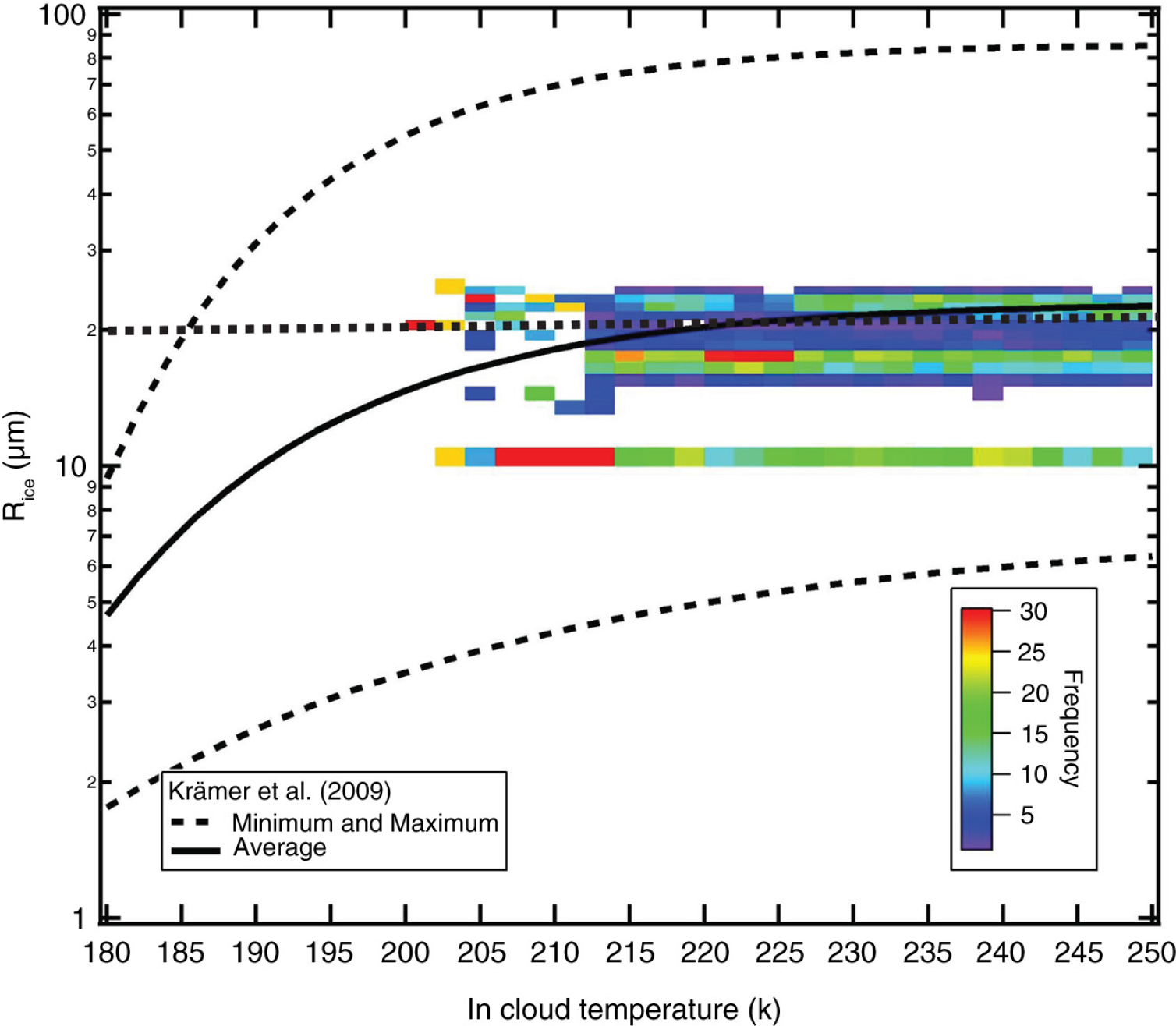
Fig. 6
This figure is the same as Fig. 4 except the average particle radius, R i, is shown as a function of temperature. The solid and dashed lines represent the median, minimum and maximum radii as a function of temperature from the data set compiled by Krämer et al. (2009). The black dotted line is the BCP median R i.
In Fig. 4, the colour of each pixel of the image plot represents the frequency with which a particular IWC–temperature pair was encountered from the total population of more than 19 000 clouds. The lower and upper dashed and solid black lines are the minimum, maximum and median values of IWC that Schiller et al. (2008) calculated for their composite data sets from 12 field projects in the Arctic, mid-latitudes and tropics over a temperature range from 183 to 250 K. Unlike Schiller et al., who constructed their figures using every one-second cloud sample, we use the size distribution at maximum concentration in each cloud to derive the IWC, as well as the N i and R i .
At temperatures colder than 230 K, the BCP measurements lie within the range shown by Schiller et al. (2008). At warmer temperatures, a larger frequency of the BCP clouds had smaller IWC than found in the Schiller et al. data set. This is not an unexpected result given that the instrument used in Schiller et al. measures the total ice water content over crystals of all sizes whereas the upper size threshold of the BCP is 90 µm. Warmer cirrus clouds will typically be composed of ice crystals covering a larger size range than found in colder clouds (Dowling and Radke, 1990; McFarquhar and Heymsfield, 1996) so that the BCP will underestimate the IWC when a significant fraction of the ice mass is found in sizes larger than 90 µm. Nevertheless, the good correspondence between the BCP measurements and those of Schiller et al. at temperatures below 225 K suggests that the majority of the ice mass at these temperatures is in crystals less than 90 µm in size. The BCP's highest frequencies lie below the median IWC from Schiller et al. This difference can be attributed to the different way that clouds are sampled during a field experiment compared with those along commercial flight tracks. During research flights, the pilot or scientific observer will visually locate the most optically thick region of a cloud to make the measurements whereas the samples taken from commercial flights will be approximately random as the pilot will maintain a prescribed course that intersects clouds by chance. Deviations only occur if the flight crew is vectored around potentially hazardous cloud systems or if they take evasive action based on their own observations. From the perspective of developing a climatologically representative database of cirrus measurements, it can be argued that the random sampling by commercial aircraft is less biased than measurements made in selected clouds during field campaigns. The avoidance by these aircraft of high reflectivity clouds, however, may produce a bias that favours clouds with lower IWC.
Another difference between the BCP-derived IWC and those of Schiller et al. is that in the BCP measurements there is not an obvious temperature trend in the median IWC whereas the median IWC of Schiller et al. increases with temperature. The BCP measurements, although showing a maximum IWC that increases from 10 ppmV at 210 K to more than 1000 ppmv at 250 K, have a median value that is approximately constant at 4 ppmV (black dotted line in Fig. 4).
Figure 5 illustrates the relationship between the maximum N i and temperature using the same colour-coding scheme as in Fig. 4 to show the percent frequency. The lower and upper black dashed and solid lines are the minimum, maximum and median values of N i as a function of temperature derived from the composite measurements by Krämer et al. (2009) taken during 28 flights in tropical, mid-latitude and Arctic field experiments in the temperature range 183–240 K. The BCP measurements fall within the Krämer et al. minima and maxima; however, the median value is constant at c.a, 0.1 cm−3, a value that is slightly less than the Krämer et al. value of 0.3 cm−3. Even though the BCP measurements do not cover the same cloud temperature range as those from Krämer et al., the important aspect to note is that neither of the data sets show that N i is related to temperatures warmer than 210 K, that is, the median N i remains constant. As with the IWC, there is an increase in the frequency of higher concentrations with temperature, that is, the maximum concentrations increase from 10 cm−3 at 210 K to more than 100 cm−3 at 250 K.
The average R i as a function of temperature is shown in Fig. 6 for comparison with the minimum, maximum and median values discussed in Krämer et al. (2009). The scale on the Y-axis is set to the same used by Krämer et al. who used the composite measurements from two instruments that covered a size range from 1 to 1000 µm, compared to the 5–90 µm range of the BCP after applying the inversion. Note that the BCP values for R i lie within the envelope of Krämer et al. (2009). Also, the 20-µm median value from the BCP (black dotted line) corresponds well to those of Kramer et al. (solid black line in Fig. 6) at temperatures greater than 210 K.
Figure 7a and b summarises the number and mass concentrations as a function of EOD for five temperature ranges. There are two features of note that change with temperature: the number and mass concentrations in the peaks and the shape of the size distributions. The concentrations increase with temperature with the exception of the interval between 210 and 230 K when there is little change observed. The size distributions are bi-modal with peaks at 18–20 µm and 43–45 µm. The bi-modality is more pronounced in the mass distributions because of the sensitivity to the cube of the EOD. In the temperature range 240–250 K, there is a hint of a third mode that is not seen at the colder temperatures.
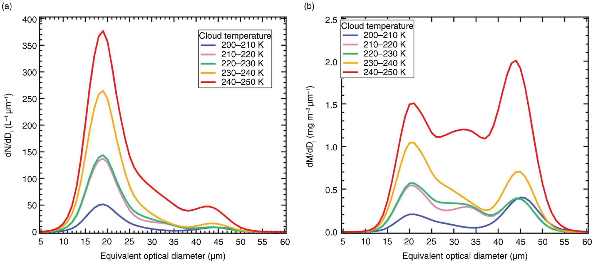
Fig. 7
This figure illustrates the (a) number and (b) mass size distributions as a function of five temperature ranges for the same cloud events used to construct Figs. (4–6).
There are many papers that report aircraft measurements in cirrus; however, few of them show size distributions in addition to the derived parameters IWC, N i and R i ; hence, it is difficult to directly compare the spectra shown in Fig. 7 and those from other studies. The measurements made during the CEPEX, reported by McFarquhar and Heymsfield (1996), cover the size range from 2 to 800 µm but the published size distributions only start at 10 µm. Nevertheless, all the distributions show a distinct peak at 20 µm. Locating the other mode in that study at 45 µm is more difficult because this mode is in the size range between the two instruments that were used to create the plots in the CEPEX study, the single particle light scattering Forward Scattering Spectrometer Probe (FSSP-100, 2–47 µm) and the 2D-C optical array probe (25–800 µm). The other studies, for example, de Reus et al. (2009), Davis et al. (2010) and Frey et al. (2011), show size distributions that are composites of two instruments, the Droplet Measurement Technologies cloud droplet probe (CDP) and cloud imaging probe (CIP), whose size ranges overlap between 30 and 50 µm. Hence, if there is a distinct mode, such as that seen in Fig. 7a and b, it is masked by the inherent uncertainties of the light scattering and optical array probes. While it is possible that the inversion technique used in the BCP analysis might be introducing this second mode, with no other co-located, independent measurement from another instrument, this cannot be verified.
A well-known uncertainty that limits the accuracy of all airborne cloud measurement instruments is susceptibility to ice crystal shattering. The cloud particle instruments all have extended arms that can produce ice fragments when crystals strike and shatter on them (Field et al., 2006a, 2006b; Korolev et al., 2011, 2013; Jackson et al., 2014; Korolev and Field, 2015). Numerous studies have been conducted to evaluate the magnitude of this effect and to develop methods to mitigate the problem (Field et al., 2006a, 2006b; Korolev et al., 2011, 2013; Jackson et al., 2014; Korolev and Field, 2015). Other studies have made convincing arguments that in most cirrus clouds, when the largest fraction of ice crystal sizes is less than 100 µm, the contribution of shattered particles is minimal (Krämer et al. 2009; Frey et al., 2011). As discussed by Beswick et al. (2014), the BCP, although completely flush with the skin of the aircraft, can also suffer from ice crystal shattering if the particles collide with the nose of the aircraft and produce secondary particles that are subsequently measured by the instrument. The magnitude of this uncertainty has not yet been evaluated but arguments similar to those made by Krämer et al. (2009) can be made that such measurement artefacts are unlikely to be significant until ice crystals larger than 100 µm are present in large concentrations.
The asphericity of ice crystals introduces an uncertainty that stems from the assumption of sphericity that is made when using the Mie theory to derive particle size from the single particle light scattering probes (BCP, CDP, FSSP). This assumption leads to undersizing of ice crystals to a degree that depends on their morphology and the orientation when they are measured. Borrmann et al. (2000) proposed a sizing correction for measurements of aspherical particles; however, this requires a knowledge of the shape of the crystals being measured and cannot be applied to the BCP data.
Figures (4–7) summarise the cirrus microphysical properties as a function of temperature regardless of cloud type, location or season. The statistics for N i , MVD, R eff and B ext are tabulated in Table 3 as a function of cloud type and season. As with the cloud size and temperature parameters listed in Table 2, the statistics presented in Table 3 are the second and third quartiles (median and 75% quantile).
Table 3. Cloud microphysical properties
To summarise, there is no consistent pattern in the relationships between the microphysical bulk properties and the season of the year. The most likely reason for this lack of consistency is that the measurements here were made at many different locations around the world. Previous studies have shown that cirrus properties are often quite different depending on where they are made, that is, the tropics, mid-latitudes or polar latitudes (Schiller et al., 2008; Krämer et al., 2009; Luebke et al., 2013). We have already observed that the IWC, N i and R i do not appear to be correlated with temperature as previous studies would suggest; hence, if there are seasonal or latitudinal relationships between these properties, they are being masked by combining them into a single data set. In the following section, we partition the data into six groups to highlight the seasonal differences by region (indicated by the boxes in Fig. 3).
3.3. Cirrus regional properties
The regions selected for further analysis were chosen to represent cirrus in the maritime (Region 1) and continental (Region 2) extratropics (40°–65°), maritime (Region 3) and continental (Region 4) tropics (from −25° to 25°) and mixed maritime–continental (Regions 5 and 6) tropics. These regions do not correspond exactly to the previous domains used by Schiller et al. (2008), Krämer et al. (2009) and Luebke et al. (2013); however, not only do the BCP measurements cover similar latitude bands, they sample many more clouds over a much broader region within these bands than was possible with the targeted research projects. Most research aircraft have a limited range due to the heavy instrument payload they carry and because field projects are typically conducted from a fixed location. Thus, the clouds that can be sampled must be within 2 or 3 hours of flight time from the site (~2000 km at typical airspeeds) to allow the aircraft to return to the home base. Commercial, long-haul aircraft, however, will cover four to five times that distance flying between two airports.
Table 4 lists the medians and third quartiles for the same derived microphysical properties as are listed in Table 2, but partitioned by region, as well as by thin and opaque cloud types. The SVC is not included in the evaluation because the aircraft encountered such thin clouds only in Regions 5 and 6. The majority of clouds were sampled in Region 5 (4339) followed by Regions 6 (619), 3 (199), 2 (110), 4 (98) and 1 (25). Figures 8 and 9 further compare the cloud properties region by region and by season.
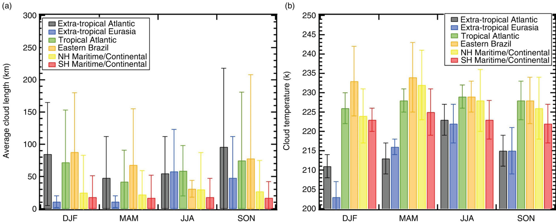
Fig. 8
The seasonal variation of (a) the average cloud size and (b) cloud temperature are summarised in this figure for the six regions. The vertical bars represent the standard deviations about the average.
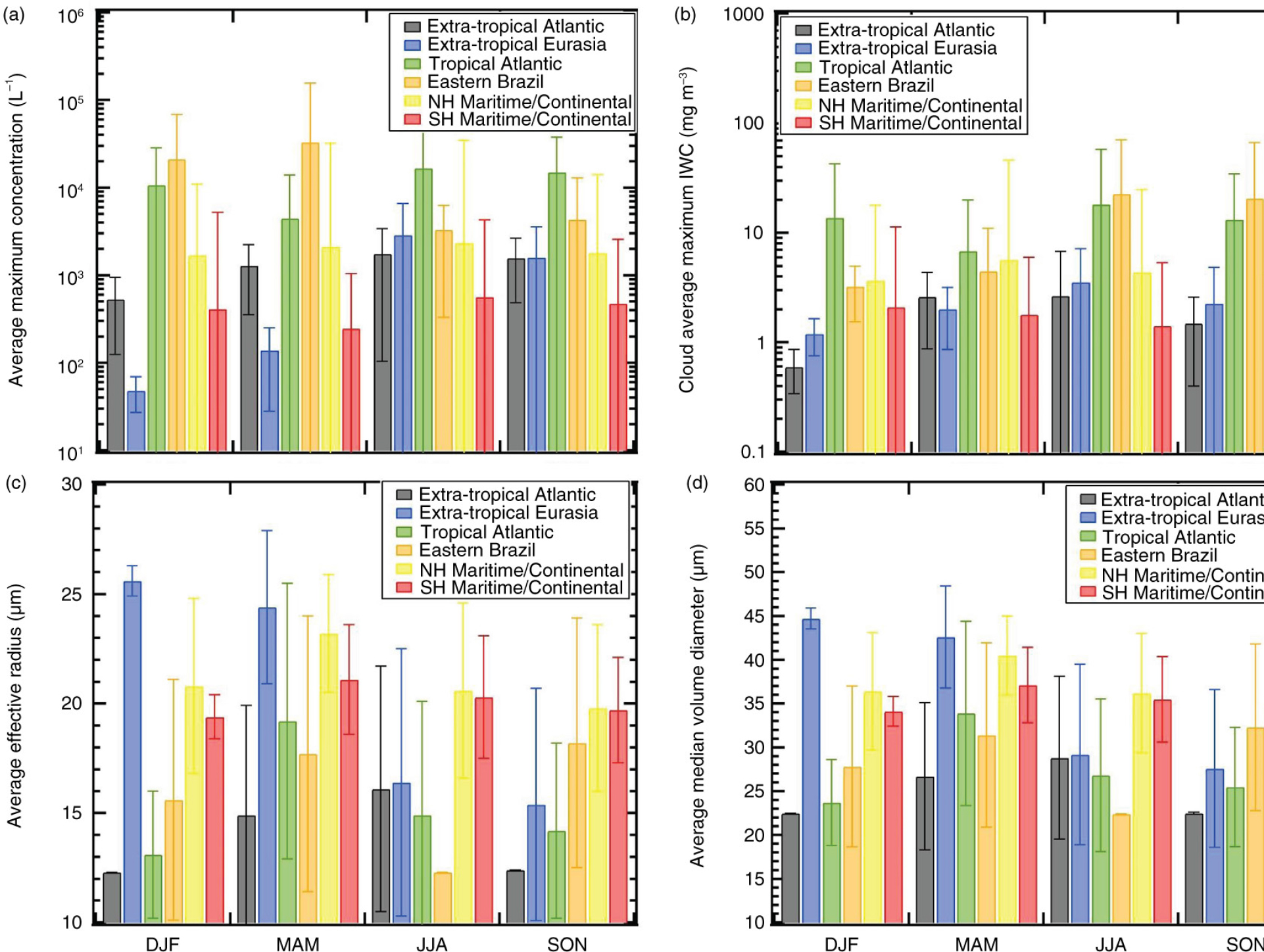
Fig. 9
This figure is similar to Fig. 8 but for the seasonal variations of the (a) average maximum number concentration (b) ice water concentration (c), effective radius and (d) median volume diameter.
Table 4. Microphysical Properties of Clouds by Region
Regions 3 and 4, the tropical maritime and continental regions, have much higher median number and mass concentrations and extinction coefficients than the other four regions, more than a factor-of-two greater, dominated by the opaque clouds. The Southeast Asia and New Guinea maritime continental clouds had the lowest concentrations but the largest effective radii and median volume diameters, 19.5 and 34.5 µm, respectively, compared to 12.5 and 22.5 µm averaged over the other four regions.
Looking at Fig. 8a and b, we observe that there are large seasonal and regional variations of average cloud size and temperature. The maritime continental clouds were the smallest over all seasons, whereas the extratropical Eurasian clouds in the summer and fall (JJA and SON) were more than five times their average size in the winter and spring (DJF and MAM). This underscores the seasonal differences in cloud formation processes. The summer and fall months are periods of heavy convection that leads to widespread cirrus formed from the outflow of such systems. The winter and spring cirrus cloud formations are driven more by frontal lifting and cold fronts that force vertical motions as they advance. The extratropical and tropical Atlantic and the Eastern Brazil regions have more pronounced seasonal cycles, but they are out of phase with one another by one season. That is, the average cloud size in the extratropical Atlantic region increases monotonically from a minimum of 50 km in the Northern Hemisphere spring, to a maximum of 100 km in the fall then decreases to 80 km in the winter. In the tropical Atlantic region, the minimum of 30 km is found in the Southern Hemisphere Winter, increasing to a maximum of 80 km in the summer before decreasing to 60 km in the fall. The Eastern Brazil region has the same trend as the tropical Atlantic but with less of a difference between the minimum and maximum. In the extratropical Atlantic, as with extratropical Eurasia, the size of the cloud is driven by the deep convection in the warm weather months and by Arctic fronts during cold weather. The trends are also more pronounced over the ocean when the outflow of extratropical cyclones that transition from tropical hurricanes in the fall.
As illustrated in Fig. 8b, the extratropical regions show the largest seasonal trends in cloud temperature, increasing from a minimum of approximately 205 K to a maximum of 225 K. The tropical regions show some seasonality but any significant changes are masked by the large standard deviations.
Figure 9a–d presents the seasonal and regional averages and standard deviations for N i , IWC, R eff and MVD. The regional differences among these microphysical properties reflect what is shown in Table 4 except that in the figure all cloud types are combined and the data are partitioned by season. Tropical Atlantic and Eastern Brazil regions dominate N i and IWC and the Southeast Asia and New Guinea regions have, on average, the larger values of R eff and MVD. As with the cloud size and temperature, the tropical regions do not have an appreciable seasonal trend whereas the minimum and maximum values in extratropical regions have significant seasonal swings; however, the extratropical Eurasia trends are quite different from their Atlantic counterparts.
All four of the microphysical parameters vary in the same manner with the minima occurring in fall and winter and maxima appearing in spring and summer. This variation is in synch with the cloud temperature trends seen for this region in Fig. 8b. The N i and IWC values in the Eurasia region are also correlated with the cloud temperature trends and follow those of the extratropical Atlantic, although the difference between the minimum and maximum values is greater over the continent than over ocean.
The extratropical Atlantic size parameters, R eff and MVD, have strikingly different seasonal changes than seen in any of the other regions, decreasing from maximum values of 26 and 45 µm, respectively in the winter, to 15 and 27 µm in the autumn. This almost factor-of-two difference in size is linked to differences in cirrus formed from summertime deep convection and from wintertime frontal systems or synoptic waves. A more comprehensive explanation of the processes that can lead to different ice crystal average sizes is beyond the scope of the current study; however, the most likely reason for the difference in crystal size is related to the rate at which air masses are lifted to form the cirrus. In the summer, when deep convection outflow is the major source of cirrus, strong vertical updrafts in the convective cores activate cloud droplets that freeze and constitute the majority of ice crystals found in the outflow. Most of their growth occurs in the early stages of formation and high water vapour supersaturations that decrease rapidly as the air exits the convective cloud and mixes with the much drier air in the upper troposphere. These smaller crystals are most abundant in the summer (Fig. 9a). In the winter, the air masses are lifted by cold fronts with a vertical motion much slower than in convective clouds. This leads to activation of fewer crystals that have a longer time to grow to larger sizes than found in convective clouds.
Figure 10 shows the mass size distributions to highlight the microphysical features that are sensitive to regional and seasonal changes. Each of the six regions exhibits distinctive seasonal shifts with respect to where the mass is distributed as a function of size. In the tropical Atlantic (Region 3), the mass spectra are mono-modal with an EOD peak of 20 µm during the summer (DJF) and spring (SON). They develop a second mode at 45 µm in the autumn (MAM) and winter (JJA). Although also in the tropics and near the tropical Atlantic region, the Eastern Brazil region size distribution is bi-modal during all seasons except summer. The bi-modality is most pronounced in the austral winter and spring. In addition, the size distribution for this region during spring is much broader around the 20-µm peak than during other seasons or over any other region. The springtime size distribution also has the hint of a third mode between 25 and 35 µm that is possibly related to the biomass burning that can predominate the aerosol particles during that period. Since biomass particles have been identified as good ice nuclei (IN), these could contribute to the formation of cirrus crystals in the outflow of deep convection.
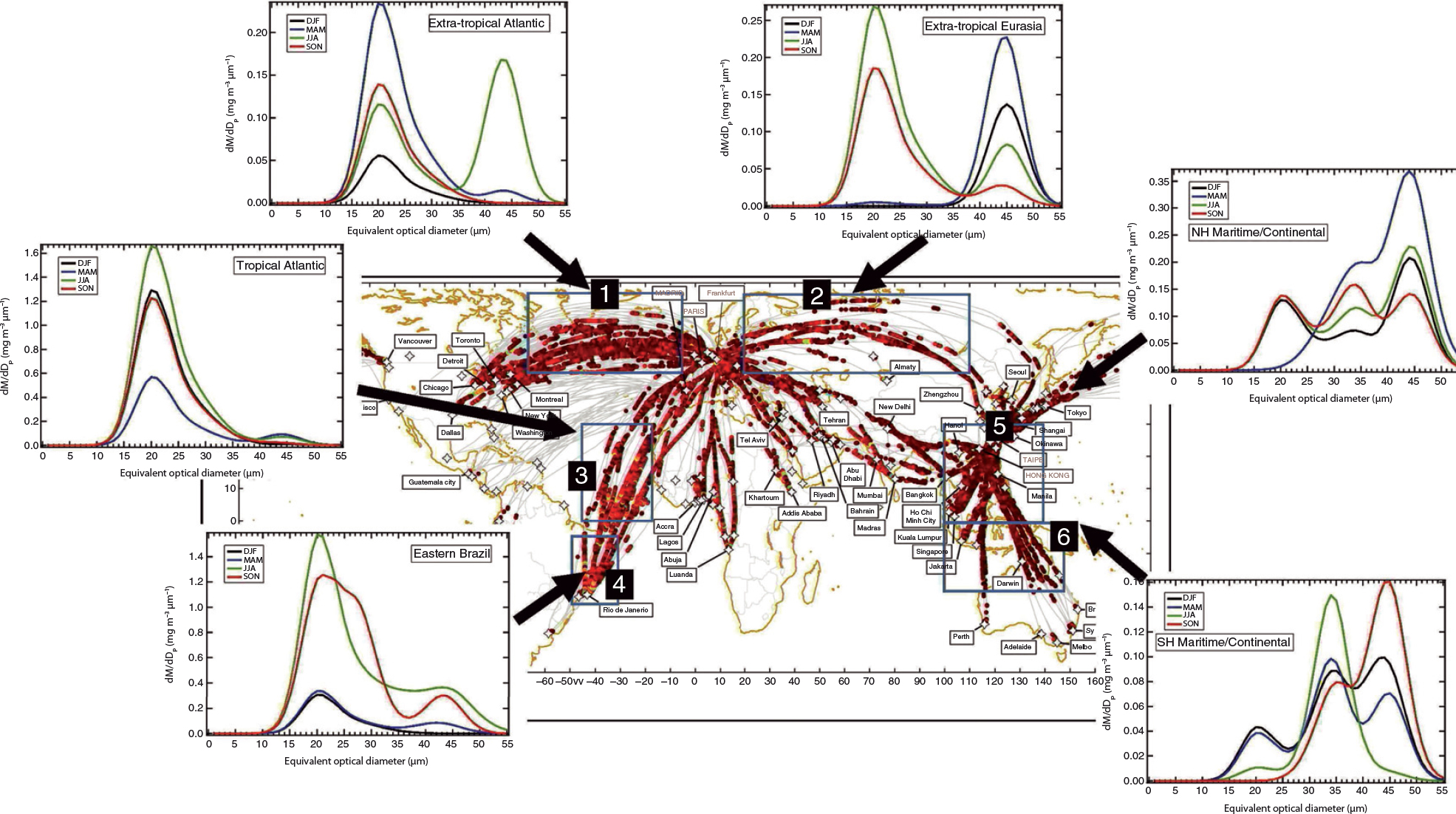
Fig. 10
The average size distributions of the mass concentrations are shown here for the six geographic regions measured over all cirrus clouds in December, January and February (black), March, April and May (blue), June, July and August (green) and September, October and November (red).
The maritime and continental extratropical regions 1 and 2 have distinctly different seasonal trends as was discussed previously when comparing the average values in Fig. 9. The Atlantic fall and winter spectra have identical shapes although the peak concentrations differ by roughly a factor of three. In the springtime, however, a second mode at 45 µm begins to develop and becomes the dominant mode in the summer. The trend in extratropical Eurasia is only mono-modal in winter with the peak at 45 µm. The 20-µm mode develops in the spring and becomes the dominant mode during the summer and autumn.
The maritime continent size spectra, in Regions 5 and 6, deviate significantly from the other four regions as they have tri-modal shapes in the summer and fall with modes at 20, 35 and 45 µm. In winter, the New Guinea size distribution collapses to a nearly mono-modal spectrum with a peak at 35 µm while in Southeast Asia there is still a hint of a peak at 35 µm; however, most of the particles are in the 20- and 45-µm modes. In spring, both regions have an almost identical shape with a shoulder at 35 µm and a maximum at 45 µm. The underlying processes that lead to these size distributions are complex. Given that these regions are both tropical, the source of the ice crystals is mostly deep convection; however, the complexity in the spectral shapes is a result of the age of the cloud when the aircraft sampled it. More in-depth satellite analysis will help to identify cloud age but again, this is beyond the scope of the present study. Another factor that may be leading to the trimodality is biomass burning, similar to what was observed in Region 4 over Eastern Brazil and that produced IN that can form cirrus ice crystals.
In summary, when evaluating the microphysical properties of cirrus clouds, seasonal changes will be masked if the data are not separated into geographical regions. It is not sufficient to look at latitudinal differences alone as the size spectra shown in Fig. 10 illustrate that clouds located in the same latitude bands can have very different distributions of mass with respect to size and will vary quite differently with season.
3.4. Comparison with other studies
In addition to the comparison of BCP measurements with the climatological data sets of Schiller et al. (2008), Krämer et al. (2009) and Luebke et al. (2013), the summer, regional number, surface and mass size distributions were compared with those from the studies of Frey et al. (2011), as shown in Fig. 11a–c. Only the summer size distributions are selected since the West Africa Monsoon study was conducted in August. From this comparison, we see that the parameterised size distributions are broader than the BCP measurements and the first mode of the BCP is twice or three times larger than the parameterised first mode. The largest mode in the BCP distributions, that fall between 30 and 50 µm, depending on the region, is very similar to the larger particle mode for the parameterisation in the potential temperature range from 355°C to 365°C. The longer tail of the parameterisation towards the larger sizes produces more surface area and mass beyond about 40 µm than measured with the BCP. The comparison with measurements made in West Africa in a particular month (August), which does not coincide with any of the six regions analysed in this study, is only shown to provide another validation of the measurement technique, complementary to what was done with the climatology comparison. For the same reasons as given in that section, the comparison with size distributions demonstrates that the shapes and relative magnitudes of the spectra are comparable to what have been measured using other research-grade instruments that cover a larger size range. The comparable magnitudes between the data sets is the only expected agreement, given the large variability observed in the different regions sampled for this study and shown in Fig. 10 that highlights the regional and seasonal differences observed.
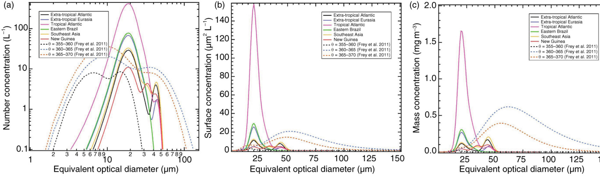
Fig. 11
The parameterised size distributions of (a) number, (b) surface and (c) ice water content, from Frey et al. (2011), are compared here with the regional spectra averaged over the summer flights.
4. Implications for flight operations
It is well recognised by the aviation industry that flight operations can be seriously compromised as a result of flying under conditions of high ice crystal concentrations (Lawson et al., 1998a, 1998b; Mason et al., 2006). In particular, ingestion of large quantities of ice crystals by jet engines can lead to a condition known as engine rollback, in which thrust reduction is caused by accumulation of ice crystals in the engine's compressor section (Mason et al., 2006). In a study of 46 such rollback events, it was discovered that the pilots had reported a total air temperature (TAT) anomaly, that is, a temperature reading much warmer than ambient (Mason et al., 2006). As shown in Fig. 12, ice crystals that enter aircraft temperature (Fig. 12a) and airspeed (Fig. 12b) sensors are melted by the inlet heaters and form liquid water that wets the temperature sensor or clogs the pitot. In the former case (Fig. 12a), the resultant reading is erroneous because the water that wets the sensor is warmer than the environment and leads to temperature readings considerably higher than ambient. In the case of water in the airspeed sensor (Fig. 12b), the total pressure will be lowered if the water completely obstructs the inlet and the derived airspeed will be underestimated. If the static ports become covered with water or ice, the indicated airspeed will increase. In either case, the true airspeed (TAS) will be erratic and cause for concern for the flight crew.
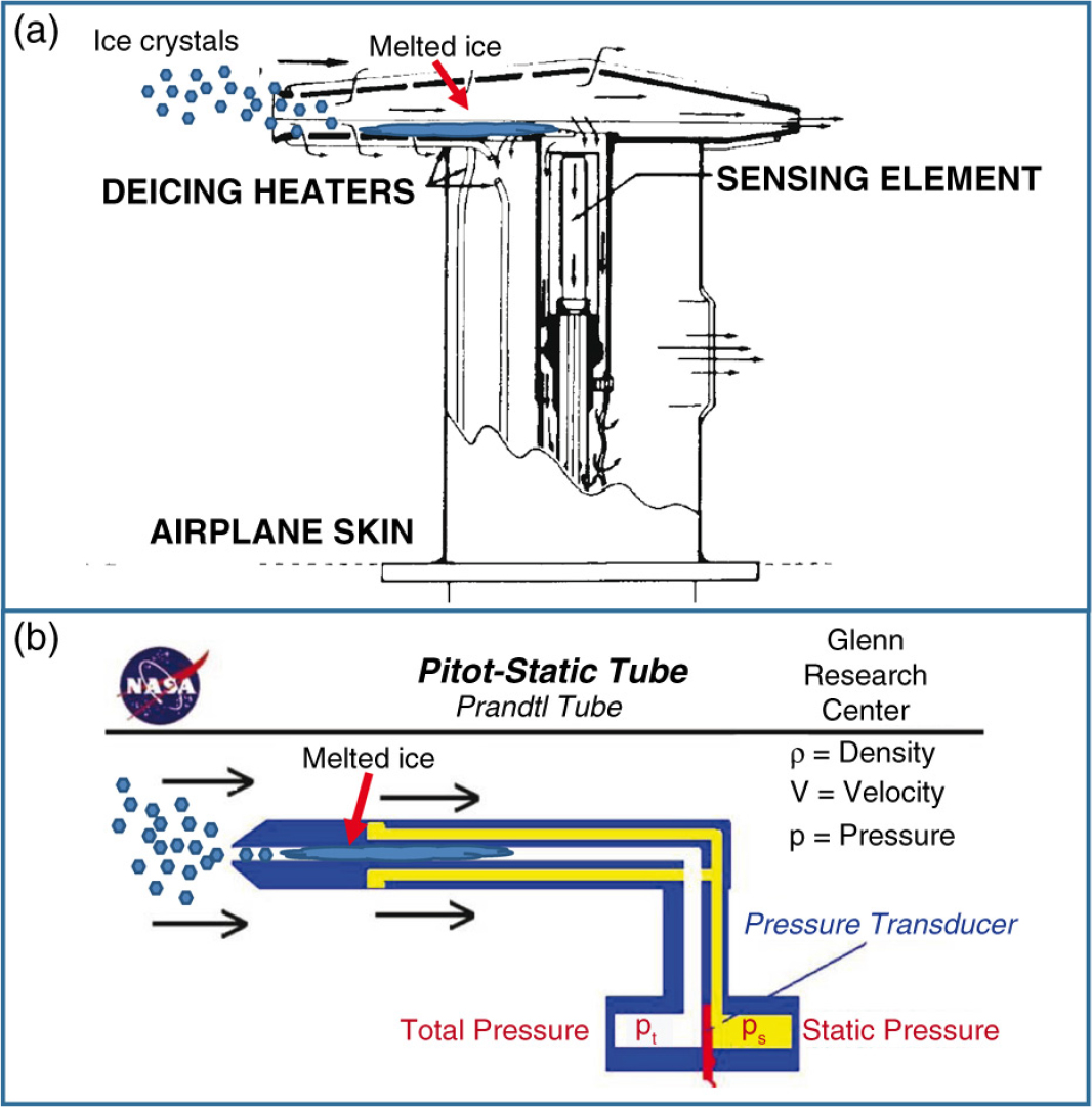
Fig. 12
As shown in these diagrams, (a) the aircraft temperature sensor and (b) airspeed sensor are susceptible to interference from high concentrations of ice crystals that enter the inlet and are melted by the sensor heaters, subsequently contributing to erroneous measurements.
Temperature and TAS anomalies were observed many times during IAGOS flights. One such encounter happened during a flight from Rio de Janeiro to Frankfurt around 0330 UTC on 14 December 2012. Figure 13 shows the 0300 UTC infrared (1) and brightness temperature difference (BTD) (2) images from Meteosat-9 with the aircraft flight path superimposed. The colouring on the BTD image corresponds to the differences between the equivalent brightness temperatures from the water vapour and infrared channels. Very small values of BTD (reds and maroon in the image) correspond to very deep convective clouds having large ice water paths (Minnis et al., 2012). Figure 14a shows a time series of N i and the air temperature during the longer segment in the cloud shown in Fig. 13. Figure 14b shows the IWC and TAS over the same time period. Note that the temperature readings are from the IAGOS sensor that is mounted at the same location as the BCP, whereas the TAS sensor is the one used by the aircraft flight system.
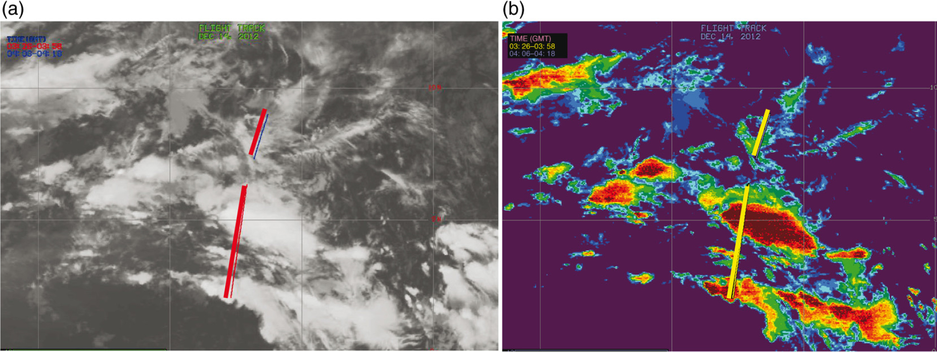
Fig. 13
The flight track of the aircraft through the clouds on December 14, 2012 is shown on the (a) visible and (b) brightness temperature difference (BTD) images from Meteosat-9. The BTD is the difference between the water vapour and infrared intensities.
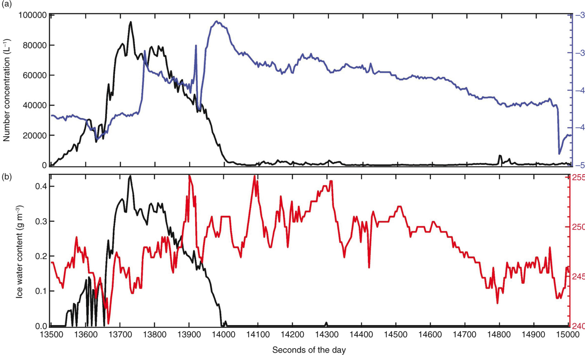
Fig. 14
Time series of (a) number concentration (black) and temperature (blue) and (b) ice water content (black) and airspeed (red).
The N i and IWC reach maximum values of 100 000 L−1 and 0.42 g m−3, respectively, values that are several orders of magnitude larger than most thick cirrus (see Figs. 4 and 5). The temperature measured as the aircraft enters the cloud is −46°C, increasing to −31° by the time the plane exits. After the aircraft exits the cloud, the sensor requires more than 15 minutes before recovering and measuring the same temperature as when it entered the cloud. This indicates that sensor, even though heated, could not evaporate the accumulated water until travelling almost 250 km beyond the cloud.
In Fig. 14b, the TAS (red curve) is seen to initially decrease by 10–240 m s−1 at the same time that the IWC increased to over 0.2 g m−3 and number concentration to more than 60 000 L−1. Following the decrease, the velocity varies wildly in a way that cannot be attributed to actions taken by the flight crew. The TAS does not return to its original value until the temperature also recovers to ambient. The wide swings in the TAS indicate that not only was the total pressure inlet obstructed but the static ports must have also been suffering from blockage that the heaters were incapable of clearing until well beyond the cloud.
As pointed out by Mason et al. (2006), in the 46 engine rollback events that were investigated, the pilots were unaware of the high ice crystal concentrations, primarily because their weather radars were not showing reflectivities that would indicate hazardous conditions. Mason et al. (2006) emphasise that high ice crystal events usually occur in large concentrations of very small crystals whose radar reflectivity (Z) is very small due to the relationship of Z~D 6. Figure 15 shows the average size distribution of the ice crystal population during the cloud pass shown in the satellite images (Fig. 13) and time series (Fig. 14). The number and mass distributions are centred on a mode of ~20 µm, a size that would produce a very low radar signal even at the observed high number concentrations.
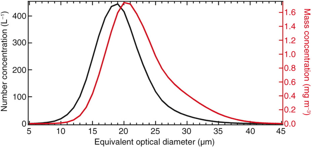
Fig. 15
This is the average size distribution of the number (black) and mass (red) concentrations during the high ice crystal event shown in Fig. 14.
These types of anomalies are not rare. In Fig. 16 the yellow filled circles show all the temperature anomalies greater than five degrees on the aircraft flight routes. There are clearly some regions of the world where these types of encounters occur more regularly than others. More than 60% of the 22 recorded anomalies, occurred over the tropical Atlantic, Southeast Asia or New Guinea.
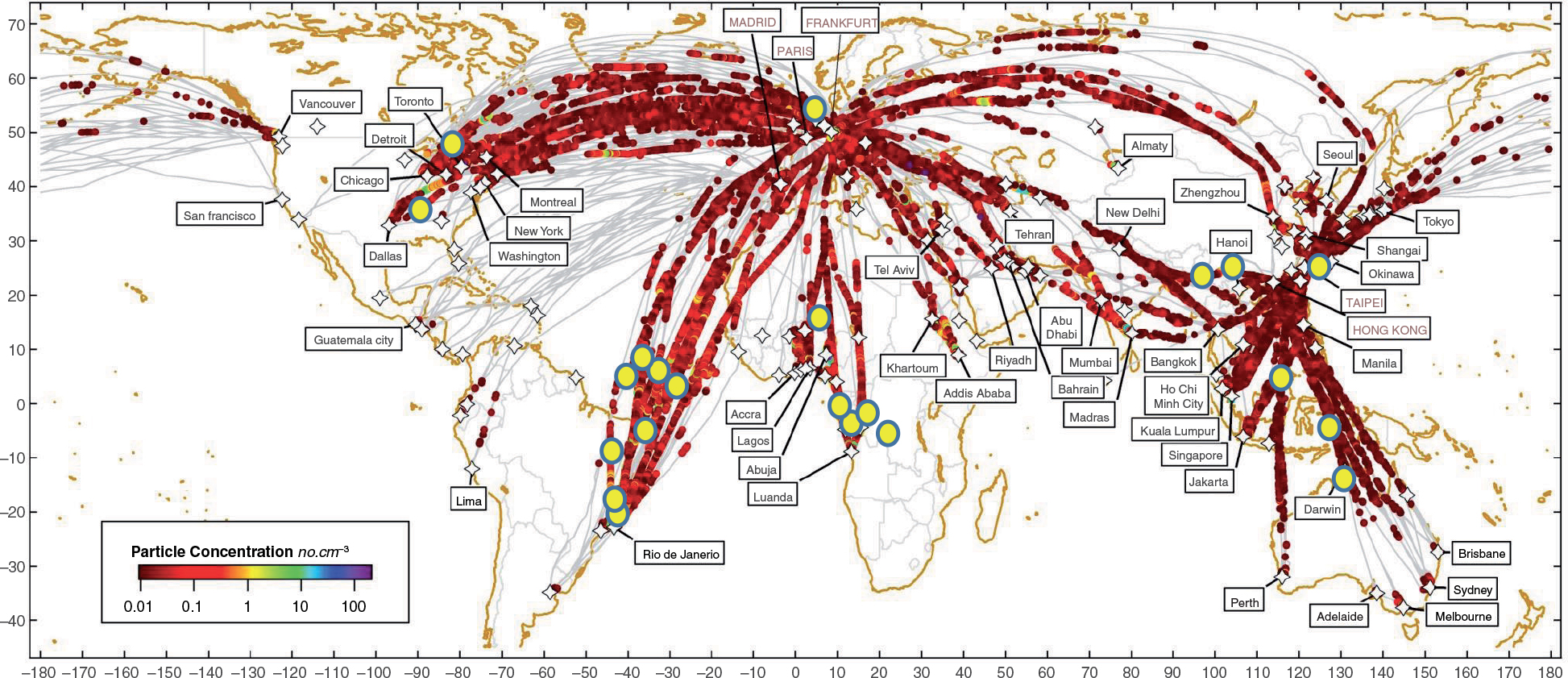
Fig. 16
There were 22 temperature anomalies recorded during the three years of measurements from 2012 to 2014. The yellow filled circles indicate temperature anomalies of greater than 5°C.
5. Summary and outlook
The analysis of size distributions from more than 19 000 cirrus clouds over a 3-yr period shows large seasonal and regional differences in the cloud physical and microphysical properties. These data were obtained from a backscatter cloud probe (BCP) mounted on five commercial aircraft that flew international routes covering four continents and latitudes ranging from 40°S to 70°N as part of the IAGOS instrument package. The BCP measures the intensity of light scattered from individual particles that pass through its laser beam and derives an equivalent optical diameter (EOD) over the size range from 5 to 90 µm from which the number concentration, N i , ice water content, IWC, effective radius, R eff, and median volume diameter, MVD are calculated.
The relationships between IWC, N i , and average radius, R i , and temperature were compared with previous studies from more than 20 airborne field campaigns that targeted cirrus in tropical, Arctic and mid-latitudes. The BCP measurements fell within the envelope of measurements that had been compiled from the field experiments. The median IWC and N i from the BCP were smaller than the medians from the field projects but the R i medians were approximately the same. The difference in the IWCs can be attributed partially to the smaller size range of the BCP compared to the research instruments that could measure the water content over almost the full range of crystal sizes found in a cloud. The difference in the N i values is due to how clouds are sampled in field projects compared to the sampling from instrumented commercial aircraft. In the former case, flight scientists or flight crews visually select the thickest part of a cirrus cloud to sample thus optimising the probability of measuring the highest concentrations. Commercial aircraft, on the other hand, are flying prescribed routes from which they rarely deviate except to avoid potentially hazardous clouds. Hence, clouds are, for the most part, intercepted purely by chance by commercial aircraft so that the BCP data set can be considered to be a truly random sampling that might be more generally representative of cirrus clouds than those that are sampled in field experiments. The upper size threshold of 90 µm measured by the BCP limits its capacity to measure the ice mass in larger ice crystals that are sometime found in warmer cirrus and ice crystals in anvil outflow; however, a survey of the literature on in situ cirrus measurements indicates that the majority of cirrus have their ice water mass in crystals with EODs that are in the range of the BCP. Analysis of size distributions parameterised from another study suggests that 20% of the surface and mass was missed by the BCP in less than 15% of the clouds sampled.
The median and third quartile of the microphysical properties of the cirrus clouds showed only small seasonal variations when averaged over all data points, regardless of the cloud type. However, when the measurements were partitioned into six regions, there were distinct differences. The regions analysed were (1) extratropical Atlantic, (2) extratropical Eurasia, (3) tropical Atlantic, (4) Eastern Brazil, (5) maritime continental Southeast Asia and (6) maritime continental New Guinea. The results show that the size distributions differ significantly between regions in the same latitude band and, within a region, there can be large seasonal variability. The size distributions of cirrus particles over the extratropical Atlantic are distinctly different than those over extratropical Eurasia. The shift in the modes of the size spectra depends on the season, reflecting the differences in the processes that form cirrus in the summer versus the winter. Likewise, cirrus over Southeast Asia and New Guinea have tri-modal distributions that are not found over any of the other regions.
The results from the seasonal and regional analysis illustrate that cirrus properties cannot be generalised by latitude band or temperature since there are clear differences that will be related to specific times of the year and local meteorology. In addition, although field experiments are needed to better characterise cirrus properties with a large suite of research instrumentation, measurements from the IAGOS systems provide a broader and more random sampling approach that will be valuable for improving climate models and refining satellite retrieval algorithms.
The results from this study have also shown that commercial aircraft frequently fly in conditions that are not identified as hazardous by their weather radars but encounter clouds having very high ice crystal concentrations that can result in obstruction of temperature and airspeed sensors. This instrument interference can cause anomalous readings that may affect the safety of the aircraft. There were a total of 22 incidents of anomalous temperature readings associated with high ice crystal concentrations during the three years. This at first appears insignificant, that is, approximately one incident per aircraft per year; however, five aircraft is less than 0.01% of the fleet of airplanes that fly yearly, suggesting that temperature anomalies and encounters with high ice crystal concentrations occur on a very regular basis.
The set of data being collected by the BCP continues to expand as the current fleet of five aircraft is still measuring clouds, while additional aircraft with IAGOS instrumentation are being added to and improved. The analysis presented in this study demonstrates that the database of cloud microphysical properties contains a wealth of information that will continue to improve our understanding of cloud processes and their impact on climate.
Acknowledgements
The authors thank the National Centre for Atmospheric Sciences, Natural Environment Research Council, United Kingdom for their support of the IAGOS project and the lead author, to Martina Krämer and Anna Luebke of the Forschungszentrum Jülich, Institut fur Chemie und Dynamik der Geosphäre 1: Stratosphäre, the NASA High Ice Water Content Program, the European Commission who supported the preparatory phase of IAGOS (2005–2012), the partner institutions of the IAGOS Research Infrastructure (FZJ, DLR, MPI, KIT in Germany, CNRS, CNES, Météo-France in France and University of Manchester in United Kingdom, ETHER (CNES-CNRS/INSU) for hosting the database, and the participating airlines (Lufthansa, Air France, China Airlines, Iberia, Cathay Pacific) for the transport free of charge of the instrumentation. They acknowledge the helpful comments and recommendations of two anonymous reviewers that help strengthen the general content of this manuscript.