
1. Introduction
Tropospheric ozone (O3) is a secondary pollutant, produced through complex photochemical reactions involving volatile organic compounds (VOCs) and nitrogen oxides (NO and NO2, referred to collectively as NOx) that are emitted from anthropogenic and natural sources (Seinfeld and Pandis, 2006). Ozone pollution raises serious environmental concerns due to its detrimental impacts on human health (Bell et al., 2004), the terrestrial ecosystem (Wang and Mauzerall, 2004) and the greenhouse effect (IPCC, 2013).
Vegetation, especially forest ecosystems, plays a crucial role in the tropospheric O3 budget by acting as the primary source of biogenic volatile organics (BVOCs). Globally, the natural emissions of non-methane VOCs exceed anthropogenic sources by nearly an order of magnitude, accounting for 90% of the total VOC inventory (Benkovitz et al., 2004). Moreover, many BVOC species are highly reactive, and they can therefore significantly influence tropospheric chemistry and composition (e.g., concentrations of O3 and secondary organic aerosols) via a series of reactions with atmospheric oxidants [e.g., hydroxyl radical (·OH), nitrate radical (NO3·) and O3] (Hallquist et al., 2009; Monks et al., 2009). The importance of BVOC emissions in O3 production has been highlighted in many megacities: for example, Paris (Solmon et al., 2004), Seoul (Kim et al., 2013), Houston (Li et al., 2007), Shanghai (Han et al., 2005) and Guangzhou (Wang et al., 2008), where anthropogenic NOx emissions are usually abundant and O3 formation is sensitive to VOCs (i.e., VOC-limited); BVOC emissions were reported to contribute 10–30% to surface O3 in these urban areas. Additionally, a group of nitrogen-fixing plants (e.g., leguminous crops) are linked to substantial soil emissions of NO, another important participant in ozone photochemistry (Wang et al., 2005). In eastern China, soil NO emissions can increase or decrease surface O3 by as much as 10–20 ppb, depending on the relative availability of NOx and VOCs (Wang et al., 2008).
Field measurements indicate that the emission capacities of natural VOCs and NO may vary by orders of magnitude depending on species composition, even among the same plant function type (PFT) (Guenther et al., 1996a; Kesselmeier and Staudt, 1999; Geron et al., 2006; Karl et al., 2009). Generally, broadleaf forests and shrubs have high emission potentials for isoprene, the most abundant BVOC species, whereas crops and grasses are considered to be low BVOC emitters. Forests around the globe are undergoing rapid changes as a result of human forces, including urbanisation, energy demand and land management, as well as natural factors such as climate change (Ramankutty and Foley, 1999; Sleeter et al., 2012). Rapid switches in plant communities could considerably modify the emissions of reactive compounds and, in turn, impact tropospheric ozone chemistry. In southern Asia, the cultivation of oil palm, due to increasing bioenergy demand, resulted in an increase in surface O3 by up to 11% (Ashworthet al., 2012); on the unpolluted island of Borneo, however, the increased BVOC emissions acted as a net chemical sink for O3 and largely reduced surface O3 and ·OH radical concentrations by 20 and 70%, respectively (Warwick et al., 2013). In China, inter-annual variations of BVOC emissions (15–28%) lead to 2–5% differences in summer O3 concentrations (Fu and Liao, 2012). Deforestation in Africa is expected to cause an increase in soil NO emissions (+9%) and a decrease in isoprene emissions (−12%), jointly resulting in a 9 ppb increase of O3 and a doubling in ·OH radical concentrations (Ganzeveld et al., 2010).
The Pearl River Delta (PRD) region located in Guangdong province of southern China is one of China's three largest urban agglomerations. Ozone pollution continues to be a critical air-quality issue in PRD, with surface O3 concentrations frequently exceeding national standards (Huang et al., 2005; Zhang et al., 2008). The PRD region is characterised by strong BVOC emissions, as a result of high forest coverage and its warm subtropical climate (Zheng et al., 2010; Wang et al., 2011). It is also thought to be the most sensitive region to BVOC emissions, which may account for up to 50% of O3 peak concentrations (Wei et al., 2007; Cheng et al., 2010).
In the last few decades, dramatic changes in the landscape have occurred in southern China (Liu et al., 2005; He et al., 2007; Liu and Tian, 2010). Based on historical archives, He et al. (2007) found that there was continuous forest restoration in China during 1978–1995, stimulated by the sustainable land policy, with an absolute increase of forest coverage rate by over 10% in Guangdong. Analyses of Landsat Thematic Mapper (TM) observations also show that the forest area in southern China expanded by 3.2×10⁴ km2 over 1980–2005 (Liu and Tian, 2010). These land-cover changes are expected to cause large variations in natural emissions and consequently O3 production.
In this study, the Weather Research and Forecasting/Chemistry (WRF/Chem) modelling system, coupled with dynamical vegetation data sets derived from Moderate Resolution Imaging Spectroradiometer (MODIS, 2001–2012) and Advanced Very High Resolution Radiometer (AVHRR, early 1990s) measurements, were used to investigate the impacts of land-cover changes on natural emissions and O3 production in PRD over the past two decades. The numerical modelling system and experimental designs are described in Section 2. Section 3 then discusses the changes in natural emissions and their impacts on O3 production. A summary and conclusion are provided in Section 4.
2. Methods and data
2.1. WRF/Chem modelling system
WRF/Chem is an online, three-dimensional, Eulerian chemical transport model that considers the complex physical and chemical processes of the atmosphere, such as emission, dry and wet deposition, advection and diffusion, gaseous and aqueous chemistry, aerosol chemistry and dynamics (Grell et al., 2005).
The WRF/Chem model is configured with a two-nested grid system that has horizontal grid spacings of 12 and 4 km, and grid points of 92×82 and 94×88, respectively (Fig. 1). The outer domain covers southern China and extends into the South China Sea. The inner domain focuses on the PRD region that contains nine cities – Guangzhou, Foshan, Zhongshan, Dongguan, Shenzhen, Zhuhai, Huizhou, Jiangmen and Zhaoqing – in addition to Hong Kong and Macao. The National Centers for Environmental Prediction (NCEP) 1°×1° final analysis data (FNL) for 2006 were used as the meteorological initial and boundary conditions. The initial chemical conditions were taken from outputs of the previous model cycle. A 12-h spin-up time was allowed, following the recommendations of Berge et al. (2001), to minimise the influence of initial conditions.
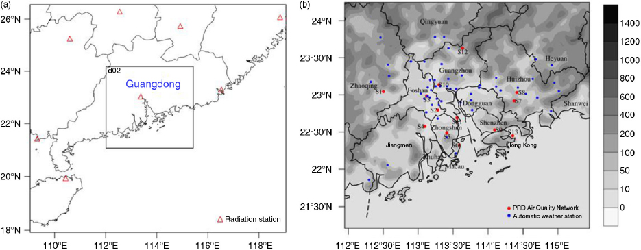
Fig. 1
(a) Two-nested WRF/Chem modelling domains and radiation observational stations (red triangle), (b) Locations of the automatic weather sites (blue dots) and air-quality monitoring sites (red dots) in the inner domain. The background shaded contour in (b) represents topography height (m); the labelled cities in (b) represent main administrative districts in the inner domain; the 13 air-quality monitoring sites are labelled as: S1 – Chengzhong, S2 – Shunde, S3 – Huijingcheng, S4 – Donghu, S5 – Zimaling, S6 – Tangjia, S7 – Jinguowan, S8 – Xiabu, S9 – Liyuan, S10 – Luhu, S11 – Wanqingsha, S12 – Tianhu and S13 – Tamen.
The key chemical modules used in WRF/Chem contain the CBM-Z gas-phase mechanism (Zaveri and Peters, 1999) and the MOSAIC aerosol module (Zaveri et al., 2008). The CBM-Z scheme was revised from the earlier CBM-IV mechanism (Gery et al., 1989) that was developed for urban applications, to treat additional reactions under low-NOx conditions (i.e., background troposphere, rural continent, and remote marine) for regional and global applications (Zaveri and Peters, 1999). It includes 52 chemical species and 132 gas-phase reactions, 7 of which are specific for isoprene chemistry. Terpene chemistry is not treated individually in the CBM-Z scheme, with higher terpenes mapped to multiples of isoprene.
The CBM-Z mechanism has been rigorously tested against chamber data and shows good performance. For example, Zaveri and Peters (1999) intercompared several lumped gas-phase chemical mechanisms – CBM-Z, CBM-IV and RADM2 (Stockwell et al., 1990) – using smog chamber experiments of Simonaitis et al. (1997) with low-NOx concentrations, as well as box models under a variety of hypothetical scenarios; they found that CBM-Z and RADM2 predicted similar O3 concentrations, both of which were in much better agreement with smog chamber data (±20%) than those produced by CBM-IV under both urban and rural scenarios. Evaluations of CBM-Z with surface O3 and NO2 concentrations observed in PRD (as in Section 3.1) also found that it showed good capacity to match actual observations.
Other physical parameterisation options include the Noah land surface scheme (Ek et al., 2003), the Lin microphysics scheme (Lin et al., 1983), the Grell cumulus parameterisation (Grell and Devenyi, 2002), the Yonsei University (YSU) boundary layer scheme (Noh et al., 2003), the Goddard short-wave radiation scheme (Chou and Suarez, 1999), the Rapid Radiative Transfer Model (RRTM) long-wave radiation scheme (Gallus and Bresch, 2006) and the Monin–Obukhov surface similarity scheme (Monin and Obukhov, 1954).
Gridded and speciated anthropogenic emissions for the outer domain were prepared using the 0.25°×0.25° Multi-resolution Emission Inventory in China (MEIC) for the year 2008 (www.meicmodel.org/), which includes all major anthropogenic sources (power plant, industry, agriculture, transportation and residential fuel), excluding biomass burning. The PRD regional emission inventory in 2006 developed by Zheng et al. (2009b) for different source categories (power plant, industry, transportation, residential fuel and biomass burning), based on activity data collected from annual statistical books, was incorporated into the inner domain. Inventory inputs of open-field biomass burning in 2006 for both domains were updated by several recent studies of our research group, based on MODIS fire products: crop residue emissions by Huang et al. (2012) and forest/grassland fire emissions by Song et al. (2009).
2.2. MEGAN natural emission model
Biogenic VOC (Guenther et al., 2006; Sakulyanontvittaya et al., 2008) and soil NO (Williams et al., 1992) emissions were calculated online using the Model of Emissions of Gases and Aerosols from Nature ver. 2.04 (MEGAN ver. 2.04) that has been incorporated into WRF/Chem. Emission rates of BVOC species, including isoprene, monoterpenes (e.g., α-pinene and β-pinene), sesquiterpenes and other volatile compounds (e.g., acids and aldehydes), were calculated and then lumped into CBM-Z mechanism species. In the following analyses, only emissions of the dominant BVOC species (i.e., isoprene, α-pinene and β-pinene) were presented to represent the total BVOC emissions.
Natural emissions are influenced by many factors, including plant composition, ambient temperature and radiation, biomass density, and leaf development. Net emission fluxes (mg m−2 h−1) for BVOCs and NO into the above-canopy atmosphere are specified empirically using a simple parameterised canopy environment model according to eqs. (1) and (2):
where EFBVOCs (mg m−2 h−1) is the canopy-scale emission factor of BVOCs, which represents the emission rates under standard conditions (e.g., normally at an air temperature of 303 K and a photosynthetic photon flux density of 1500 µmol m−2 s−1). EFNO (mg m−2 h−1) is the emission factor for soil NO that is dependent on land-use category. Deviations of BVOC emissions from standard conditions are modified through a set of dimensionless activity factors to represent the impacts of air temperature (γ T), photosynthetically active radiation (γ P), leaf area index (LAI, γ LAI), leaf age (γ age), soil moisture (γ SM), light dependence (LDF) and production/loss within the canopy (ρ) [eq. (1)]. Detailed calculations for each correction term can be found in Guenther et al. (2006) and Sakulyanontvittaya et al. (2008). For soil NO emissions, only the influence of soil temperature (T s) was considered [eq. (2)].
In this study, PFT-specific emission factors of BVOCs for the four aggregated PFTs (i.e., broadleaf forest, coniferous forest, shrub, and cropland/grassland) were determined by local field observations in the literature (Guenther et al., 2006; Sakulyanontvittaya et al., 2008; Tsui et al., 2009; Leung et al., 2010; Wang et al., 2011). NO emission factors from soil were developed through measurements with static or dynamic chambers (Williams et al., 1992; Guenther et al., 2000). The PFT and LAI data sets for the vegetation were provided from satellites (see Section 2.3). Meteorological outputs of temperature, radiation and moisture from WRF were used to estimate the activity factors of biogenic emissions.
2.3. Experiment designs
Four land-use scenarios (Table 1), designated as ‘MEGAN90’, ‘MEGAN01’, ‘MEGAN06’ and ‘MEGAN12’ were used to reflect the natural emissions in the early 1990s, 2001, 2006 and 2012, respectively. All four land-use scenarios were configured with identical parameterisation schemes and anthropogenic emissions, NCEP FNL meteorological inputs for 2006, as well as the same chemical initial/lateral boundary conditions, as described in Section 2.1. The land surface parameters, derived from MODIS remote sensing in 2006, were updated in the WRF weather model for all four simulations, as described in our previous work (Li et al., 2014). However, these simulations have different representations of PFTs and LAI for the estimation of natural emissions in MEGAN, as described below.
Table 1. Experimental designs and input data
The MEGAN06 case is regarded as a base simulation, in which MODIS measurements for the year 2006 were used to describe the distributions of PFTs and LAI. The MODIS sensors aboard Terra (1999.12 − ) and Aqua (2002.05 − ) satellites gathered data in 36 spectral bands, seven of which are designed for vegetation monitoring. The 500 m MODIS land-cover product (MCD12Q1), generated through a supervised decision-tree classification method (Friedl et al., 2002), was used to construct the PFT data set. The MODIS LAI data (MCD15A2), with a spatial resolution of 1 km and an 8-day temporal resolution (Garrigues et al., 2008), were resampled on a monthly basis and then used as inputs to estimate the influence of LAI (γ LAI) and leaf age (γ age) on BVOC emissions. Similarly, MODIS satellite retrievals for the years 2001 and 2012 were used in MEGAN01 and MEGAN12, respectively, except that LAI in MEGAN01 was substituted with MODIS measurements for 2003 because of data missing (Table 1).
The other case (MEGAN90) was designed to represent natural emissions in the early 1990s, using PFT and LAI data sets that were derived from AVHRR measurements made by the Polar Orbit Environment Satellite (POES) (Loveland et al., 2000). The 1-km IGBP DISCover (International Geosphere – Biosphere Programme Data and Information System) global land-cover map, which was acquired from monthly AVHRR NDVI (Normalized Difference Vegetation Index) observations spanning from April 1992 to March 1993 (Loveland et al., 2000), was chosen to represent the PFT distribution. The 15-day, 8-km LAI generated from historical observations of AVHRR NDVI in 1992 was used in this experiment (Liu et al., 2012).
In addition to the direct effects of land-cover changes on natural emissions through modifying EFs, γ LAI and γ age, meteorological factors (mainly temperature and radiation) are also important determinants of BVOC emissions (Geron et al., 2006). To distinguish the impacts of initial meteorological conditions on BVOC emissions, taking the period from 2006–2012 as an example, another simulation, ‘METE12’ was also conducted. In the METE12 simulation, NCEP FNL data for 2012 were used as the meteorological inputs for WRF/Chem; PFT and LAI data sets from MODIS satellite retrievals for 2006 were used in MEGAN, which were the same as those in MEGAN06 (Table 1). Moreover, land surface is the fundamental interface for land–atmosphere interactions, and thus changes in surface physical properties associated with land-cover changes can also modulate boundary layer meteorology and in turn BVOC emissions (Ganzeveld et al., 2010). To reflect the responses of BVOC emissions to meteorological variations induced by land-cover changes, a sixth simulation (‘MELU90’) was run, using land surface parameters derived from AVHRR measurements in the early 1990s in the WRF meteorological model (Li et al., 2014). Detailed experiment designs and input data for all six simulations are provided in Table 1.
Previous studies (Zheng et al., 2010; Wang et al., 2011) suggested significant seasonal variations in natural emissions, with a peak in summer owing to strong solar radiation and higher temperatures. Thus, this study focuses on the summertime impacts of land-cover changes on O3 production, using a month-long simulation lasting from 1 to 31 July 2006.
3. Results and discussions
In the following sections, model outputs of meteorology, atmospheric composition (O3 and NO2 concentrations) and BVOC emission fluxes in the base case (MEGAN06) are used for model validation. The decadal variations in natural emissions and O3 concentrations are also analysed with respect to model outputs of the MEGAN06 simulation.
3.1. Model validation
3.1.1. Meteorology
The meteorological data used for model validation included hourly observations of 2-m air temperature, 2-m relative humidity and 10-m wind speed/direction obtained from 72 automatic ground stations throughout the inner domain (Fig. 1b) and daily radiation measurements at eight stations in the outer domain provided by the National Meteorological Information Center (Fig. 1a). The meteorological model results are compared against actual observations using mean bias (MB), root mean square error (RMSE), fractional bias (FB), fractional error (FE) and index of agreement (IOA) (Table 2).
Table 2. Performance statistics of simulated meteorological variables in MEGAN06
The WRF/Chem model performance was well within the typical ranges of mesoscale models (Hanna and Yang, 2001; Li et al., 2014). Slight underestimation of 2-m temperature was seen, with a cold bias of −0.31°C and RMSE of 2.02°C. In terms of 2-m relative humidity, the simulations have high moist bias (5.18%) and RMSE (11.64%). Generally, model overestimation of surface wind speed is evident (0.99 m s−1) during the modelling period. A high positive bias in wind speed has also been reported by several other studies using WRF/Chem (Matsui et al., 2009; Molders et al., 2012; Tuccella et al., 2012; Li et al., 2014), which may be because it is difficult to resolve weak winds realistically in the current generation of mesoscale models and topographical features in surface drag parameterisation (Cheng and Steenburgh, 2005; Zhang et al., 2015). Mean angular differences between the simulated and observed wind directions are within 80° and an MB of 17.46° is seen across the inner domain (Table 2). Simulated short-wave radiation is significantly larger than observations, with an MB of 82.83 W m−2. The large radiation overestimation (over 60 W m−2) has also been noted in previous studies (Wang et al., 2011; Situ et al., 2013), and can be attributed, at least in part, to model inaccuracies in gas/aerosol-radiation feedback.
3.1.2 O3 and NO2
Hourly ground-level O3 and NO2 concentrations collected at 13 air-quality monitoring stations in the PRD air-quality monitoring network (Fig. 1b) were used for model evaluation of chemical composition.
The magnitudes and diurnal/daily trends for O3 concentration were reasonably well predicted at most network sites (Fig. 2), with an overall correlation coefficient of 0.73 and normalised mean bias (NMB) of 30%. The O3 levels generally peaked at 13:00–16:00 LST (local standard time) and were at a minimum in the morning and nighttime due to O3 titration loss and deposition (Seinfeld and Pandis, 2006). At most sites, O3 concentrations appeared to be overestimated by 10–30%. The simulation overestimation of summertime O3 is thought to be a common problem over East Asia due to the inability of the model to accurately represent cloud cover and monsoon rainfall, as well as inadequate representation of southerly inflow of clean marine air masses (Lin et al., 2009; Chatani and Sudo, 2011). In particular, the modelled O3 is quite poor on some rainy days (e.g., 10–11, 15–17 and 26–29 July) because of model inaccuracy in precipitation. It is also noted that the O3 peak concentrations tended to be under-predicted at a few upwind rural sites in eastern PRD; for example, Jinguowan and Xiabu, which may be related to uncertainties in precursor emissions and transport processes due to the wind errors, as well as chemical mechanisms in the low-NOx regimes. At two other rural sites (Chengzhong and Tianhu), located downwind of PRD, simulated O3 concentrations agree well with observations, indicating that WRF/Chem generally captures rural O3 formation (Fig. 2).
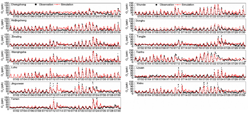
Fig. 2
Time series comparisons of the simulated O3 concentration (ppb) (red line) in MEGAN06 against observations (black dot) at 13 monitoring sites.
Comparisons of NO2 concentrations at the monitoring sites further demonstrate that O3 formation was reasonably captured (Fig. 3), with a domain-average NMB of −8% and NMB of 31%. The NO2 concentrations showed an almost opposite diurnal variation to that of O3; that is, characterised by a maximum during the nighttime and morning rush hours, and a substantial decrease in the middle of the day due to low emissions, active chemical loss, and strong turbulent mixing. Because the NO2 mixing ratio is influenced by local effects such as emissions and diffusion conditions, the model overestimates NO2 concentrations within a range of 10 ppb around the source regions (e.g., Zimaling and Tangjia) and underestimates NO2 at suburban sites (e.g., Jinguowan and Xiabu).
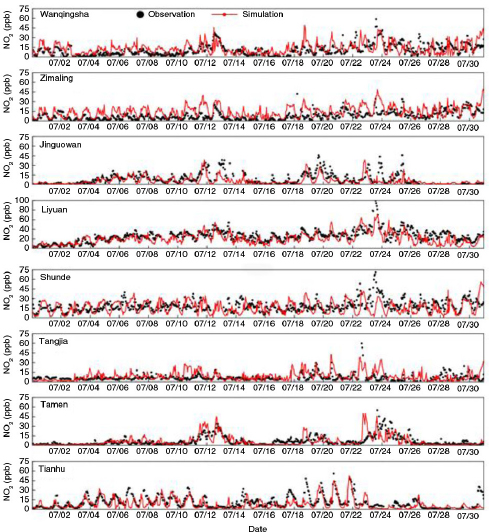
Fig. 3
Time series comparisons of the simulated NO2 concentration (ppb) (red line) in MEGAN06 against observations (black dot) at eight representative sites.
3.1.3 BVOC emissions
Available observations of BVOC emission fluxes (Gao et al., 2011) and ambient concentrations (Bai and Wang, 2001) in the literature were used to evaluate the MEGAN model estimates of BVOC emissions in this study.
Using the Relaxed Eddy Accumulation (REA) technique, Gao et al. (2011) conducted canopy-scale measurements of isoprene fluxes on sunny days at a litchi (lychee) plantation (114.76°E, 22.98°N) located in northeastern PRD in July 2008. In the present study, the estimated daytime (06:00–18:00 LST) isoprene emission flux at this site ranges between 0.11 and 0.24 mg C m−2 h−1 (with an average of 0.16 mg C m−2 h−1) on sunny days, which is very close to the average measured value of 0.2 mg C m−2 h−1 by Gao et al. (2011).
To further evaluate the model performance, a simple box model (Guenther et al., 1996b; Situ et al., 2013) that considers the local BVOC emission, the vertical mixing and chemical loss of BVOC species through oxidation with ·OH radicals and O3 [eq. (3)], was used to estimate the ambient BVOC concentrations.
where C is the mixing ratio of BVOC species, E is the simulated BVOCs emission flux, Z i (m) is the height of mixed-layer capping inversion and L (s−1) is the oxidation rate by ·OH and O3. L is defined as , where K·OH and are the reaction rate constants of BVOC species with ·OH and O3 reported by Atkinson and Arey (2003), and C·OH and are the simulated mixing ratios of ·OH and O3, respectively.
Bai and Wang (2001) measured the composition of non-methane VOCs at Dinghu mountain (112.53°E, 23.17°N) located in northwestern PRD, from June 1995 to August 1996. The observed daytime isoprene and α-pinene concentrations in July were reported to be within 0.4–1.0 and 0.05–0.1 ppb, respectively. The calculated isoprene and α-pinene concentrations at this site are in the ranges of 0.19–0.51 and 0.02–0.03 ppb, respectively, which are lower than observations by a factor of 1–2. Transport of anthropogenic pollutants from the nearby urban areas is another major source of non-methane VOCs at the Dinghu site, which may be in part responsible for the model underestimation.
Generally, the MEGAN model combined with high-resolution, satellite-derived PFT and LAI data tends to reasonably predict summertime BVOC emissions in northeastern PRD, and causes underestimations in northwestern PRD. However, more field experiments are needed to provide a more accurate and rigorous evaluation of BVOC emission fluxes in the PRD region.
3.2. Decadal variations in natural emissions due to land-cover changes
3.2.1. Vegetation changes by remote sensing
BVOC emissions are highly dependent on forest area. Figure 4 illustrates the inter-annual variations of forest area in Guangdong since the early 1980s, which are acquired from continuous satellite measurements by the AVRHH and MODIS sensors, along with multiple survey data sets, including the 5-year State Statistical Bureau survey data (www.stats.gov.cn/), the National Forest Survey (NFS, 1988–2002) (www.escience.gov.cn/) and the Comprehensive Monitoring of Forest Resources and Ecological State (1983–2002) (Ye, 2010), as well as the annual Bulletin of Guangdong Forestry and Ecological Environment (2004–2012) (www.gdf.gov.cn/) and the Guangdong Forestry Bureau Archives (1994–2003) (Zhou et al., 2007).
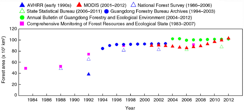
Fig. 4
Inter-annual variations of forest area (×103 km2) in Guangdong based on remote sensing and statistical surveys.
In the early 1980s, the Guangdong provincial government promulgated multiple forest conservation policies (e.g., ‘Enclosure of Hillside for Afforestation’) and laws to preserve the declining forest resources, resulting in rapid forest growth in the 1980–1990s (Fig. 4). In 1983–2002, forest area in Guangdong increased by 4.3×10⁴ km2, with an annual rate of 2.5% (Ye, 2010). In the early stage of the last decade, however, the forest ecology deteriorated slightly and forest coverage rate was reported to drop by 1.5% in 2004–2006. This lasted until the 11th Five-Year Plan (2006–2010), at which time the goal of ‘Sustainable Forestry Development’ was established and multiple forestry ecology projects and forest carbon sink programmes were launched; the forest coverage rate began to increase continuously by ~2.9% (www.stats.gov.cn/).
Generally, the MODIS sensor was able to capture the decadal variations in forest area (Fig. 4). As detected by the MODIS measurements, a slow decrease (−0.9×10³ km2 yr−1) in forest area occurred in Guangdong from 2001 to 2006, followed by continuous forest expansion by 2.9×10³ km2 yr−1 until 2012 (Fig. 4). In the three MODIS land-use scenarios, the forest area in Guangdong was 9.0, 8.6 and 10.3×10⁴ km2 in 2001, 2006 and 2012, respectively. According to the SSB and NFS field surveys, the forest coverage rate in Guangdong reached 46.5 and 49.4%, respectively, in 2006, very close to the estimated value of 47.9% from MODIS remote sensing. Particularly, coniferous forests accounted for 33.2% of the total forest area, which was similar to the field surveys (38.5%) by Ye (2010). The coverage fraction of cropland (19.7%) and grassland (13.8%) from MODIS measurements also agreed well with the SSB surveys (22.9% for cropland and 18.4% for grassland) and Landsat TM satellite observations by Liu et al. (2005) (18.7% for cropland). Previous studies also suggested that the MODIS sensor performed quite well in vegetation monitoring, with a deviation from field surveys within 5% (Ran and Li, 2006a, 2006b).
However, it is also apparent that compared with the survey data by SSB and Annual Bulletin (2004–2012), the growth rate of forest area in Guangdong over 2006–2012 may be overestimated by a factor of two. This may be partly related to the 500-m pixel size of MODIS measurements, and also to differences in forest definition and monitoring methodology between remote sensing and field surveys. The low forest coverage in the early 1990s is also visible in the AVHRR data set (3.8×10⁴ km2 in Guangdong) and remote sensing indicated a nearly doubled increase of forest area in the 1990s. Despite that, the AVHRR data set tends to seriously underestimate forest area by around 20–40%, when compared with the NFS statistical census (4.9×10⁴ km2 in 1988 and 6.5×10⁴ km2 in 1992; Fig. 4), due to the limited spectral channels and unsupervised classification (Frolking et al., 1999). Thus, MEGAN90 should be regarded as a hypothetical case, indicative of low natural emissions in the early 1990s.
The contrast map (Supplementary Fig. 1) for each PFT in these four land-use scenarios further illustrates that the terrestrial ecosystem in PRD experienced dramatic changes over the past two decades. During the early 1990s, the entire PRD region was characterised by substantial amounts of cropland (~109.4×10³ km2), which accounted for 61.9% of the inner domain. After that, an unprecedented loss of agricultural land (with lower BVOC emissions) and reforestation (with higher emissions) occurred over large parts of the mountainous areas in Huizhou and Jiangmen. Moreover, the dominant tree species in Guangdong also changed from coniferous forest (mainly strong terpene emitters) into broadleaf forest (predominantly isoprene emitters), which is consistent with that reported by Ye (2010). In the last decade, the total changes in forest cover between the base year (2006) and 2001/2012 add up to −4.4 and +16.5%, respectively. These changes in forest area are partly reflected in the domain-average LAI, with a decrease from 1.37 m2 m−2 in MEGAN01 to 1.20 m2 m−2 in MEGAN06, followed by a subsequent increase to 1.26 m2 m−2 in MEGAN12 (data not shown).
3.2.2. Decadal variations in natural emissions
As shown in Table 3, the results of this study fall within the ranges of previously published inventories in PRD (Zheng et al., 2010; Wang et al., 2011) and Hong Kong (Tsui et al., 2009). For example, in the present study the average isoprene emission flux in PRD was 0.35 Mg C km−2 in July, slightly higher than the summertime average of 0.31 Mg C km−2 reported by Wang et al. (2011). Our total isoprene emission estimate in Hong Kong (0.35 Tg C) was also close to the given value of 0.39 Tg C by Tsui et al. (2009), but both estimates were lower than the value reported by Leung et al. (2010) (1.0 Tg C) by 60–70%, due to the large differences in input data used (Table 3).
Table 3. Comparisons of isoprene emissions in MEGAN06 with previous studies
[iv] dGloBEIS refers to the Biogenic Emissions Inventory System developed by Guenther et al. (2000);
Plotted against weather conditions, modelled biogenic emissions display a bell-shaped diurnal cycle, peaking at approximately 13:00 LST and nearly ceasing overnight (particularly for isoprene), with decreasing temperature and solar radiation (Supplementary Fig. 2). Figure 5 compares the spatial distributions of average BVOC and NO emission fluxes in the four land-use experiments during 11:00–16:00 LST. The strongest BVOC emissions (>100 mol km−2 h−1) occurred in the far northwestern and northeastern rural regions of PRD, including Zhaoqing, Heyuan, Huizhou, Qingyuan and Jiangmen, accounting for nearly 80% of the total emissions.
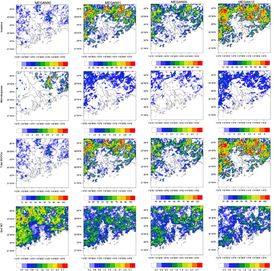
Fig. 5
Average estimated emission fluxes (mol km−2 h−1) for isoprene, monoterpenes, total BVOCs and soil NO at 11:00–16:00 LST in these four simulations. The total BVOC emission flux is expressed as a sum of isoprene, α-pinene and β-pinene.
As expected, the contrast maps of BVOC emission factors (Supplementary Fig. 3) and real natural emissions (Fig. 5) closely match the results of vegetation changes (Supplementary Fig. 1). In the early 1990s, the sparse broadleaf forests and dense coniferous forests resulted in higher monoterpene emission capacities in northeastern PRD, as well as low isoprene EFs throughout the inner domain (Supplementary Fig. 3). As a result of extensive afforestation since the 1990s, the isoprene EFs exhibited sharp increase (Supplementary Fig. 3) and 32.5 Gg C of isoprene was emitted from the inner modelling domain in July, 2006, approximately threefold that emitted in the early 1990s (11.3 Gg C). The changes in total emissions of monoterpenes (expressed as a sum of α-pinene and β-pinene) were relatively minor (3.6 Gg C in 2006 and 3.5 Gg C in the early 1990s) (Fig. 5). In the last decade, when compared with that in 2006 (Fig. 5c), BVOC emissions were slightly reduced since 2001 (Fig. 5b) and increased by up to 20–30 mol km−2 h−1 in 2012 (Fig. 5d) as the forest expanded. Overall, total BVOC emissions over the inner domain decreased by −5.8% yr−1 in 2001–2006 (−5.7% yr−1 for isoprene and −6.9% yr−1 for monoterpenes) and increased by +9.1% yr−1 in 2006–2012 (+9.2% yr−1 for isoprene and +8.0% yr−1 for monoterpenes). The land-cover changes also resulted in a different temporal distribution for soil NO emissions (Fig. 5e–h), which gradually decreased throughout the entire inner domain, owing to the loss of agricultural land. However, generally, the soil NO emissions contributed marginally to total NOx emissions in this region.
3.2.3. Changes of BVOC emissions in response to meteorological variations
In addition to the direct effects of plant composition on natural emissions, changes in boundary layer meteorology can also profoundly impact BVOC emissions and, in turn, ozone chemistry, which are not included in the discussions above. Comparisons of model output from the two sensitivity simulations (METE12 and MELU90; Table 1) could provide an insight into the isolated impacts of meteorological variations on natural emissions.
Meteorological outputs from MEGAN06 and METE12 demonstrate that the daily maximum short-wave solar radiation and 2-m air temperature in July increased from 835.6 to 900.8 W m−2 and from 31.1 to 31.5°C, respectively, during 2006–2012 (Fig. 6). As expected, the increasing solar radiation and temperature produced a ~1.1% yr−1 increase in BVOC emissions in the inner modelling domain (Fig. 6). Compared with the large increase in BVOC emissions (9.1% yr−1) due to land-cover changes, the impacts of variations in initial meteorological conditions (1.1% yr−1) may be minor. Similarly, Leung et al. (2010) analysed the inter-annual variations of BVOC emissions in Hong Kong during 1995-2006 and found a 7% yr−1 increase in BVOC emissions, attributed to land-cover changes, and a much smaller decrease (−1.4% yr−1) due to meteorological variations.
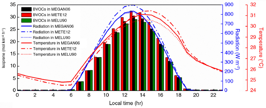
Fig. 6
Diurnal variations of solar radiation (W m−2), air temperature (°C) and BVOC emission fluxes (mol km−2 h−1) averaged over the inner domain in MEGAN06, METE12 and MELU90.
Comparisons of meteorological outputs from MEGAN06 and MELU90 (Fig. 6) find that, land-cover changes (mainly urbanisation and afforestation) in the past two decades caused a warming effect in the inner domain, which averaged 0.5°C for daily maximum 2-m air temperature and 10.5 W m−2 for short-wave solar radiation, respectively. The higher temperature and radiation were favourable for natural emissions, leading to ~2.8% increase in total BVOC emissions over the inner modelling domain (Fig. 6). Compared with the two-fold increase in BVOC emissions due to land-cover changes, the emissions adjustment by the ambient temperature and solar radiation induced by land-cover changes may be negligible. Tao et al. (2013) also found a weak increase (~3.1%) of isoprene emissions in the United States through the altered meteorological conditions induced by land-cover changes.
Thus, the discussions below focus on the direct impacts of altered BVOC emissions on O3 production attributable to land-cover changes.
3.3. Impacts of the changes in BVOC emissions on O3 production
The O3 distributions over PRD are characterised by large spatial inhomogeneity under different meteorological conditions. Depending on the daily wind regime, the 1-month simulation is classified into four categories as shown in Supplementary Fig. 4: southeast (1–3, 30–31 July) and southwest (5–9, 18–19 July) wind conditions under the influence of the prevailing East Asian Monsoon, calm wind conditions (12, 20–23 July) induced by the tropical cyclones ‘BILIS’ and ‘KAMEI’, and north wind conditions (13–14, 24–25 July) occurring after the tropical cyclones made landfall. No analysis was performed on rainy days with low O3 and natural emissions.
3.3.1. Regional and diurnal variations in 2001–2012
Impacts of the decadal changes in BVOC emissions during 2001–2012 are reflected in differences of O3 peak concentrations (ΔO3peak) between the three MODIS land-use scenarios (Fig. 7). The chemical processes controlling O3 formation depend non-linearly on the relative abundance of VOCs and NOx (Seinfeld and Pandis, 2006); thus the distributions and magnitudes of ΔO3peak vary greatly in response to the meteorology and upwind/downwind positions of biogenic and anthropogenic sources.
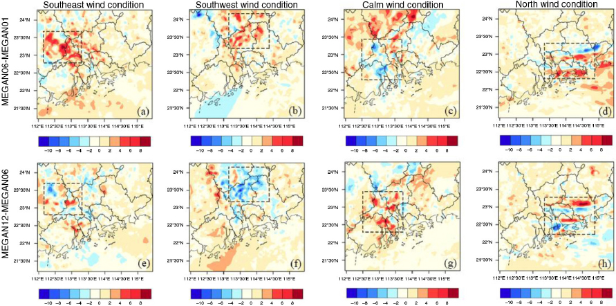
Fig. 7
Changes in O3 peak concentrations (ppb) relative to the year 2006 under different wind conditions. The dashed boxes mark the sub-domains with large ΔO3peak.
Influenced by the prevailing southerly monsoon in summer, elevated O3 (>70 ppb) usually occurs in the downwind suburban and rural areas of PRD, while the O3 concentration in urban centres is low, due to the titration effect by fresh NOx emissions (Supplementary Fig. 4a–b). Accordingly, the changes in surface O3 peak concentrations are more obvious in downwind rural areas (e.g., the outskirts of Guangzhou and Foshan, and Zhaoqing; Fig. 7). In the last decade, opposite patterns were observed in the distributions of ΔO3peak for the periods 2001–2006 (Fig. 7a, b) and 2006–2012 (Fig. 7e, f). Under the southeast wind conditions, the increased BVOC emissions in 2006–2012 reduce O3 peaks in northwestern PRD by 2–6 ppb (−1.6 ppb on average; Fig. 7e). Conversely, the slightly reduced BVOC emissions from 2001 to 2006 are projected to increase O3 peak concentrations by up to over 6 ppb (+4.0 ppb on average). Similarly, under the most common southwest wind, the increase/decrease of BVOC emissions leads to −2.5/ + 1.2 ppb changes in O3 peak concentrations in northern PRD (Fig. 7b and f). In the low-NOx rural environment (or ‘clean’ chemical regime), increased BVOC emissions and biogenic RO2 . radicals tend to react with atmospheric HO2 . radicals (Seinfeld and Pandis, 2006) and act as a chemical sink for O3, which may explain the impacts of altered BVOC emissions on rural O3 formation over the last decade.
During the calm wind conditions associated with an approaching tropical cyclone, weak winds, strong solar radiation and high temperatures are common; thus, severe and prolonged O3 pollution (>100 ppb) is observed in the central PRD (Supplementary Fig. 4c). In the vicinity of central urban areas (e.g., Guangzhou, Foshan and Zhongshan), anthropogenic NOx emissions are usually abundant (a ‘polluted’ chemical regime) and thus O3 production become sensitive to BVOC emissions, with ΔO3peak reaching as high as ±2–6 ppb (Fig. 7c, g). The increased BVOC emissions in 2006–2012 caused an average increase of 1.7 ppb in O3 peak concentration (Fig. 7c), mainly due to the enhanced conversion of NO into NO2 by biogenic RO2 . radicals (Seinfeld and Pandis, 2006). Similarly, a slight reduction in surface O3 peak concentrations, by −1.1 ppb, can be seen in the central PRD between 2001 and 2006 (Fig. 7g). Following landfall of tropical cyclones, the strong north wind moves O3 plume and its precursors to the southern coastal areas (e.g., Shenzhen and Hong Kong) and the Pearl River Estuary (Supplementary Fig. 4d), where changes in BVOC emissions affect the surface O3 concentrations more obviously. During 2006–2012, an increase in O3 peaks was modelled in Shenzhen and southern Huizhou (Fig. 7h), opposite to that during 2001–2006 (Fig. 7d).
Taking the 2006–2012 case as an example, Fig. 8 presents the diurnal variations of district-level changes in BVOC emissions (ΔBVOC) and surface O3 concentrations (ΔO3) between the two simulations. It is noticeable that, although the directions of O3 changes may differ under any wind condition, the diurnal variations in the magnitude of ΔO3 show a close correlation with that of BVOC emissions. ΔBVOC starts to increase after sunrise (around 06:00 LST), when simultaneously the photochemical activity and ΔO3 also begin to intensify. Typically, ΔBVOC (0–40 mol km−2 h−1) and ΔO3 reach a maximum at around 13:00–15:00 LST. Further diagnostic analyses (data not shown) indicate that photochemistry contributed most to the large O3 changes around noontime. ΔBVOC begins to drop and reaches a minimum after sunset (around 18:00 LST), whereas high ΔO3 can still be found during the non-photochemically active periods (e.g., morning and nighttime), which may be indicative of the transport of long-lived O3. Under calm conditions, the surface O3 enhancement (1.5–3.0 ppb) in Guangzhou, Foshan, Zhongshan and Zhuhai cities was most sensitive to the altered BVOC emissions, despite local changes in BVOC emissions being small (within ±10 mol km−2 h−1), followed by Jiangmen and Huizhou. During southwest wind conditions, Guangzhou, Zhongshan and Huizhou are the most sensitive regimes to the increased BVOC emissions, with O3 concentrations reduced by 1.0–3.0 ppb.
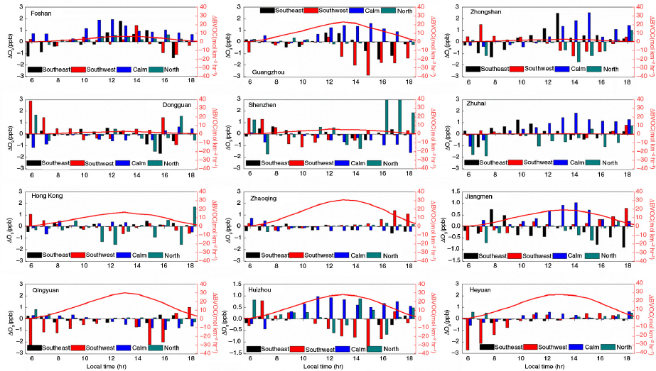
Fig. 8
Changes of the daytime BVOC emission fluxes (mol km−2 h−1) (red line) and surface O3 concentrations (ppb) (histogram) in the main cities between 2006 and 2012.
3.3.2. Variations of O3 from the early 1990s to 2006
Figure 9 presents the impacts of changes in BVOC emissions on surface O3 peak concentrations (Fig. 9a–d) between the early 1990s and 2006, and their diurnal variations (Fig. 9e–h). Under southerly wind conditions (Fig. 9a–b), the nearly two-fold increase in natural emissions acts as an important source of atmospheric RO2 .radicals and consistently enhances O3 production at the remote sites by up to 4–8 ppb. The areas with maximum O3 increases are found in the northwestern rural and suburban regions (e.g., Zhaoqing, Guangzhou and Foshan; Fig. 9a), coinciding with those featuring the strongest increase of BVOC emissions, by over 30 mol km−2 h−1 (Fig. 5). On average, the increased BVOC emissions cause an approximately 0.6–4.6 ppb increase in daytime O3 concentrations (Fig. 9e). Similarly, influenced by the southwest wind (Fig. 9b), 2–6 ppb increase of O3 peak concentrations can also be seen in northern PRD (e.g., Guangzhou and Qingyuan), leading to an average increase of O3 by 0.9 ppb on a regional scale (Fig. 9f). Under the calm and north wind conditions, the central Guangzhou and Dongguan cities (Fig. 9c), as well as the northern Shenzhen, Hong Kong and Huizhou cities (Fig. 9d) become most sensitive to the increased BVOC emissions, with maximum increments of 1.7 and 3.7 ppb in O3 concentrations at around 12:00–14:00 LST, respectively (Fig. 9g–h).
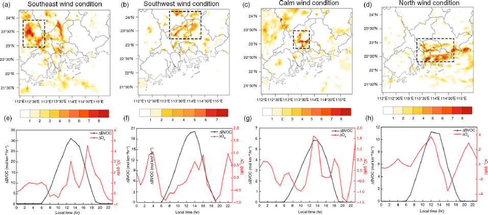
Fig. 9
(a–d) Changes of O3 peak concentrations (ppb) during the early 1990s to 2006 under different wind conditions. The dashed boxes mark the sub-domains with large ΔO3peak. (e–h) Diurnal variations of ΔO3 (ppb) (red line) and ΔBVOC (mol km−2 h−1) (black line) at the sub-domains marked in (a–d).
Similarly to those of 2001–2012, it can be seen that the diurnal variations of surface O3 concentrations also show a nearly synchronous trend with that of BVOC emissions (Fig. 9e–h), with ΔBVOC (6–30 mol km−2 h−1) and ΔO3 (0.9–4.6 ppb) maximising around noontime. In southeast wind conditions, however, the maximum increase of surface O3 (>4.5 ppb) can be seen in the late afternoon (from 16:00 to 18:00 LST), with another small peak (~3 ppb) occurring at 12:00–13:00 LST. The smaller peak around noontime accounts mainly for the photochemical influence; the occurrence of the later maximum can be attributed to the combined effects of O3 transport to this downwind area (dominant process), surface O3 accumulation caused by the decreasing boundary layer height, and O3 photochemistry. Situ et al. (2013) modelled the contributions of BVOC emissions to O3 formation in PRD; they also noted the occurrence of double peaks in the downwind edge of northwestern PRD. In southwest wind conditions, the diurnal effects on surface O3 concentrations also closely follow that of BVOC emissions, but with later maximum values (by nearly 1.0 ppb) at around 14:00–16:00 LST due to the influence of advection transport to the downwind region.
4. Conclusions
The decadal variations in natural emissions due to land-cover changes, in particular emissions of reactive BVOCs from the terrestrial ecosystem, play a key role in ozone chemistry. In this study, the WRF/Chem modelling system, coupled with continuous MODIS (2001–2012) and AVHRR (early 1990s) measurements, was used to investigate the impacts of land-cover changes on natural emissions and consequently O3 production in the PRD region over the past two decades.
Model results indicate that BVOC emissions are highly dependent on the growth and decline of forest cover in this region. The total BVOC emissions increased by a factor of ~2 since the early 1990s to 2006 due to extensive afforestation, with a slow decrease (−5.8% yr−1) in 2001–2006 and then a continuous increase (+9.1% yr−1) from 2006 until 2012. The decadal variations in BVOC emissions have complex implications for O3 production in PRD, depending on the chemical regimes and prevailing winds. The impacts on O3 production were more substantial in the downwind areas. It was found that the two-fold increase of BVOC emissions since the early 1990s to 2006 cause a 0.9–4.6 ppb increase in surface O3 concentrations over the downwind region. Since the start of the 11th Five-Year Plan, the large increase in BVOC emissions has tended to reduce the surface O3 peak concentrations in rural regions by 1.6–2.5 ppb on average, whereas it increased the urban O3 peak by up to 2.0–6.0 ppb. The opposite was true in the period 2001–2006, when the reduced BVOC emissions resulted in 1.3–4.0 ppb increases in daytime O3 concentrations over northern rural regions.
Numerous studies (Byun et al., 2005; Guenther et al., 2006; Pfister et al., 2008; Han et al., 2013) have highlighted the sensitivities of natural emissions and O3 concentrations to the input vegetation parameters. With three data sets of satellite-derived PFTs and LAI, Pfister et al. (2008) demonstrated variations in regional isoprene emissions by a factor of two or more, causing up to 5 ppb inter-deviations of O3 concentrations between these parallel simulations. The deviations of satellite-derived vegetation parameters from field surveys have been pointed out in Section 3.2. Moreover, intrinsic discrepancies also exist between the AVHRR and MODIS data sets owing to retrieval algorithms and resolution. For example, Lu et al. (2005) reported that in growing season the AVHRR LAI in China was generally larger than that from MODIS. Despite these uncertainties, the application of AVHRR/MODIS monitoring does reflect the dynamics of vegetation changes over the past two decades.
Gas-phase chemical mechanisms and emission algorithms are another source of uncertainty in this study. Comparisons of different chemical mechanisms (Hough, 1988; Jeffries and Tonnesen, 1994; Kuhn et al., 1998; Luecken et al., 1999; Zhang et al., 2012) found similar simulated concentrations of O3, but in rural regions the differences in O3 concentrations increased due to different representations of isoprene–·OH chemistry (Luecken et al., 1999; Gross and Stockwell, 2003). Particularly, monoterpenes have been shown to have a lower chemical reactivity (Atkinson and Arey, 2003) and O3 formation potentials (Carter, 1994; Poisson et al., 2001; Ortega et al., 2007; Curci et al., 2009; Zheng et al., 2009a; Cheng et al., 2010; Hellén et al., 2012) in the real atmosphere, so treating them as isoprene may over-emphasises their impacts. In the recent version 2.1 of MEGAN (MEGAN ver. 2.1), an explicit canopy environment and leaf energy balance model has been implemented, which is expected to provide more reliable BVOC estimates (Guenther et al., 2012). Moreover, an improved approach of soil NO emission (Yienger and Levy, 1995), which includes the enhancement by nitrogen (N) fertiliser application and soil moisture variations, has also been replaced in MEGAN ver. 2.1. These important features should be included in future work.
This study indicates that the potential impacts of future vegetation changes on biogenic emissions and ozone chemistry should be considered in long-term land-use planning and air-quality management. Scenarios of future land cover by Sleeter et al. (2012) and Yuan et al. (2013) indicated that the forest area in China will expand continuously in the next century, particularly in the southeastern mountainous areas. Since 2011, implementation of three key ecological forestry projects in Guangdong (i.e., forest carbon sinks, forests into cities, and ecological landscape forests) is expected to considerably promote forest plantations in the next few decades. These rapid landscape changes feature large increases in high BVOC-emitting genera such as Bambusa, Cinnamomum burmannii, Pinus massoniana, Schima superba and Acacia (Klinger et al., 2002; Geron et al., 2006), which are projected to exacerbate photochemical pollution within urban zones. To achieve optimal O3 mitigation strategies in cities, the replacement of low BVOC-emitting subtropical species, for example, Cinnamomum camphora, Bombax ceiba, Sweetgum, Castanopsis fissa, Manglietia glauca, Gmelina, and Swietenia (Klinger et al., 2002; Geron et al., 2006), may be a better alternative in urban greening. Additionally, elaborate data sets of species-level BVOC emission potentials should be established for assessment of the possible chemical consequences of land planning.
Acknowledgements
This study was supported by the National Natural Science Foundation of China (41275155 and 41121004), the Public Welfare Project for Environmental Protection (201309009), the project 2010CB428501 supported by Chinese Ministry of Science and Technology and the special fund of State Key Joint Laboratory of Environment Simulation and Pollution Control (14Y01ESPCP). The MODIS land products were provided by Land Process Distributed Active Archive Center (LP-DAAC).