
1. Introduction
Temporal variations in the mixing ratio of long-lived trace gases near the tropopause can rise slowly into the lower stratosphere (LS) via the ascending branch of Brewer–Dobson circulation (or tropical upwelling). This phenomenon was first observed in water vapour (Mote et al., 1995) and was referred as ‘atmospheric tape recorder’ by Mote et al. (1996). Subsequently, the tape recorder signal was found in other tracer gases such as carbon dioxide (CO2), carbon monoxide (CO) and hydrogen cyanide (HCN) (Andrews et al., 1999; Schoeberl et al., 2006; Pumphrey et al., 2008; Li et al., 2009; Pommrich et al., 2010). The CO tape recorder is thought to be linked to the seasonal variations of CO in the upper troposphere (UT), which are mainly driven by the seasonal variations in biomass burning (Schoeberl et al., 2006). However, Randel et al. (2007) pointed out that the CO annual oscillation (AO) in the LS is primarily induced by the annual cycle in upwelling, rather than the seasonal variations of CO in the UT. Schoeberl et al. (2008) used the MLS CO data to analyse the annual variations of CO in the tropical LS and proposed that the annual variations of the vertical component of the Brewer–Dobson (BD) circulation have an impact on the annual fluctuation of CO in the LS. As the fossil fuel and biomass burning near the Earth's surface is the primary source of CO in the troposphere, it is understandable that the CO seasonal variations are linked to biomass burning. However, the CO annual signal was reproduced by chemistry-climate model (CCM) simulations without biomass burning emissions [Fig. 10b in Jin et al. (2009)] and with a fixed CO boundary condition in the UT [Fig. 7c in Tian et al. (2010)]. This clearly highlighted the importance of dynamical processes on the CO annual cycle in the LS. Another interesting feature in the above-mentioned study is that the CO annual signal in CCM simulations with fixed CO boundary condition in the UT is more obvious than that in the MLS observations (Tian et al., 2010), suggesting that the seasonality of biomass burning may not exactly be in phase with the seasonality of the dynamical processes generating the CO annual cycle in the tropical upper troposphere and lower stratosphere (UTLS) region.
Besides the CO annual cycle above 80 hPa in the tropical LS, there is a semi-annual oscillation (SAO) near the tropopause (between 146 and 80 hPa) with the maximum amplitude at 100 hPa (Schoeberl et al., 2006; Randel et al., 2007). Schoeberl et al. (2006) argued that the CO SAO is due to the semi-annual cycle in biomass burning sources. However, Liu et al. (2007) argued that it is caused by the combination of the semi-annual variations of biomass burning and the semi-annual variations of convective overshooting (Liu and Zipser, 2005). Folkins et al. (2006) also attributed the CO semi-annual cycle at 100 hPa to the seasonal changes in dynamical processes (convective outflow and upwelling) and the seasonality of CO biomass burning emissions. Duncan et al. (2007) and Liu et al. (2013) analysed the impacts of surface emissions and transport on the temporal patterns of CO in the UTLS using chemistry-transport models and found that both the surface emissions and deep convection have an impact on CO temporal variations in the UTLS region.
It is known that the oxidation of hydrocarbons in the troposphere and stratosphere and the photolysis of CO2 in the upper mesosphere and lower thermosphere can produce CO, while the oxidation reaction with OH is the sink of CO in the whole atmosphere (Solomon et al., 1985; Minschwaner et al., 2010). The CO tape recorder signal fades out at about 40 hPa (Schoeberl et al., 2006), whereas the tape recorder signals in H2O, CO2 and HCN can rise to about 10 hPa (Mote et al., 1995; Andrews et al., 1999; Pumphrey et al., 2008). The significant different feature of the tape recorder signals between CO and the other gases is attributed to the CO 1–2 months chemical lifetime at these altitudes (Schoeberl et al., 2006). Recently, Abalos et al. (2012) emphasized that there is a balance between CO increase due to vertical transport and decrease due to photochemical loss in the LS. Hence, the chemical processes associated with CO may also have a non-negligible impact on CO temporal variations in the UTLS region.
It is apparent from the above-mentioned studies that the CO surface emissions, dynamical and chemical processes all make a contribution in generating CO temporal variations in the tropical UTLS region. But the dominant factor controlling of CO AO and SAO signals in the tropical UTLS still remains under debate. In this study, we attempt to clarify the relative importance of CO emissions, dynamical and chemical processes in generating the AO and SAO of CO in the UTLS using a CCM together with satellite observations of CO. Section 2 gives a brief description of the model and numerical experiments. Section 3 examines the ability of the model to reproduce observed tropical CO anomalies and then presents our analysis of CO emissions, CO chemical and dynamical processes in influencing the variability of CO in the UTLS. A summary is given in Section 4.
2. Model and numerical experiments
The numerical tool used in this study is the free-running WACCM (Whole Atmosphere Community Climate Model, version 3), which has 66 vertical layers from the ground to 4.5×10⁻⁶ hPa (approximately 145 km geometric altitude). The vertical resolution is 1.75 km around the stratopause (50 km), 1.1–1.4 km in the LS (below 30 km) and 1.1 km in the UT. The WACCM includes a detailed chemistry module for the middle atmosphere with a good performance in various aspects (Eyring et al., 2006; Garcia et al., 2007; SPARC, 2010). The chemistry module includes 11 reactions associated with CO (seven gas-phase reactions and four photolytic reactions), which are listed in Table 1 for reference. The convection scheme used in the model is documented by Zhang and McFarlane (1995).
Table 1. The chemical reactions associated with CO and the corresponding reaction rates in the WACCM
[i] Adopted from Sander et al. (2003).
The monthly mean CO surface emissions used in the model are based on the emission inventories described in Horowitz et al. (2003). The surface emissions are divided into four types: anthropogenic fossil fuel burning and other industrial activity (hereafter ‘anthro’), biomass burning and biogenic emissions from vegetation (hereafter ‘bb’), biogenic emissions from soils (hereafter ‘soil’) and biogenic emissions from ocean (hereafter ‘ocean’). Figure 1 shows the temporal variations of zonal mean CO surface emissions anomalies averaged over the latitude band 10°N–10°S. Here, the anomalies are defined as the departures of monthly mean CO values from its annual mean. The zonal mean CO surface emissions anomalies from ‘anthro’, ‘bb’, ‘soil’ and ‘ocean’ sources are also shown in Fig. 1. We can see from Fig. 1 that there is an evident SAO in tropical CO emissions, which is in agreement with Duncan et al. (2003). The semi-annual cycle of CO surface emissions is mainly due to semi-annual variations of ‘bb’ as shown by Horowitz et al. (2003). It should be pointed out that aircraft emissions of CO provided by Friedl (1997) are also included in the model, but there are no seasonal variations in aircraft emissions. The CO upper boundary of the model is lidded at 3.37×10⁻⁸ hPa and specified by the TIME-GCM (Roble and Ridley, 1994).
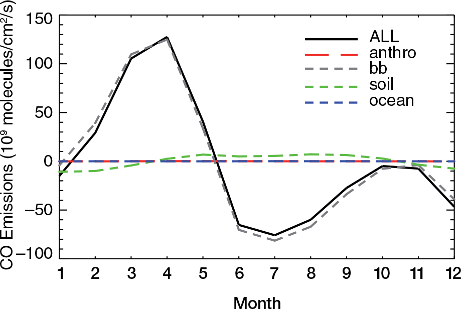
Fig. 1
Temporal variations of zonal mean CO surface emissions anomalies (solid line) averaged over the latitude band 10°N–10°S in the WACCM. The anomalies are defined as the departures of the monthly mean values from their annual mean. Also shown are the zonal mean CO surface emissions anomalies from ‘anthro’ (red dashed line), ‘bb’ (grey dashed line), ‘soil’ (green dashed line) and ‘ocean’ (blue dashed line) sources (see text for the definitions of these abbreviations).
To investigate the relative importance of CO surface emissions, the CO upper boundary, chemical and dynamical processes in affecting the CO variability in the tropical UTLS region, six numerical experiments were performed, and their basic configurations are given in Table 2. In all the simulations, the sea surface temperatures and sea-ice fractions are monthly mean values averaged over the time period from 1995 to 2000. The base run E0 is designed for verifying the model's ability of simulating the observed CO variability in the UTLS region. In run E0, the monthly mean CO surface emissions are adopted at the model's lower boundary. As the tropical quasi-biennial oscillation (QBO) can also affect the variability of tracer distributions in the tropical stratosphere (e.g. Giorgetta and Bengtsson, 1999; Baldwin et al., 2001; Schoeberl et al., 2008; Ricaud et al., 2009), a nudged QBO is forced in run E0. For the purpose of eliminating the effect of the QBO on tracer distributions, another run R0 (Total), which is the same as E0 except that the QBO is not included, is also performed. In all other sensitivity experiments, there is no nudged QBO. In sensitivity run R1 (rmEmis), the CO surface emissions are constant annual mean values, while the other configurations are the same as that in run R0 (Total). Run R2 (rmEmis+rmUb or Trans+Chem) is the same as run R1 (rmEmis) except that the seasonality of CO at the model upper boundary is removed. The chemical reactions associated with CO are included in runs R0 (Total), R1 (rmEmis) and R2 (rmEmis+rmUb). In run R3 (Trans), the CO chemical reactions are excluded by setting the chemical reaction rates of the 11 chemical reactions listed in Table 1 to zero. In run R4 (Trans+Prod), only Reaction 7 is excluded. The lower and upper boundary conditions of CO in runs R3 (Trans) and R4 (Trans+Prod) are annual mean values. The six simulations are performed at 4°×5° (latitude×longitude) resolution and run for 23 yr, with the first 3 yr of model outputs used as model spin-up, and the remaining 20 yr of model outputs used for analysis.
Table 2. The configurations of the numerical experiments
From run R0 (Total) and run R1 (rmEmis), we attempt to diagnose the contribution of the seasonality of CO biomass burning emissions to the CO temporal variations in the tropical UTLS region. From run R1 (rmEmis) and run R2 (rmEmis+rmUb), we diagnose the impact of the seasonality of the model's CO upper boundary. The impact of dynamical processes on CO is analysed from run R3 (Trans). From runs R2 (Trans+Chem), R3 (Trans) and R4 (Trans+Prod), we try to understand the impact of CO chemical processes on the CO variations in the tropical UTLS.
Apart from the model simulations, the Aura Microwave Limb Sounder (Waters et al., 2006) (MLS version 2.2 products) CO observations are used to compare with the modelled CO in base run E0. Validation of the MLS CO data has been discussed by Pumphrey et al. (2007) and Livesey et al. (2008). The useful range of CO in pressure is from 215 to 0.0046 hPa. The vertical resolution of MLS CO at these levels is ~4 km. In our analysis, the monthly mean CO mixing ratios in the 10°N–10°S are calculated from the MLS measurements from January 2005 to December 2010, and the data combining both day and night time CO measurements are binned into 4°×5° (latitude×longitude) resolution, consistent with the model resolution. The ACE Fourier Transform Spectrometer (ACE-FTS) version 2.2 CO data from 2005 to 2010 are also used to compare with the modelled CO in base run E0. Further details about the validation of the ACE-FTS CO data product can be found in Clerbaux et al. (2008). To explore the dynamical process, the monthly mean outgoing longwave radiation (OLR) for the period from 1975 to 2010 from the National Oceanic and Atmospheric Administration (NOAA; Liebmann and Smith, 1996) is also analysed. In addition, the ERA-Interim reanalysis data are used to verify that the WACCM model can reasonably simulate the circulation fields, particularly the BD circulation in the UTLS region. To diagnose the transport of tracers in the tropical UTLS region by the BD circulation, the components of the BD circulation (,) are computed from the following (Andrews and McIntyre, 1978):
where ρ is the density, ν and ω are the meridional and vertical components of the velocity, respectively, θ is the potential temperature, a is the Earth's radius and φ is latitude. In the above formula, the overbars represent zonal means, primes are deviations from them.
3. Results
3.1. CO tape recorder signal in model simulations and MLS data
Before proceeding further, a comparison of the modelled CO mixing ratios in the boreal winter with the MLS, ACE-FTS CO observations is first given in Fig. 2. Note that both the ACE-FTS CO and the modelled CO are weighted by the MLS averaging kernels to make a more accurate comparison. Figure 2 shows that the modelled CO mixing ratios are smaller in magnitude than the MLS CO and ACE-FTS CO observations in the UTLS region in DJF. However, the spatial distributions of the modelled CO are overall similar to that of the observations. The ACE-FTS observations show large CO mixing ratios in the Northern Hemisphere (NH) UT as a result of high CO surface emissions in the NH and relatively slow photochemical loss in wintertime (González Abad et al., 2011), and the model also captures this feature. The modelled CO mixing ratios in the UTLS in the other seasons show the similar feature to that in DJF (not shown). Nevertheless, it should be pointed out that most of the analysis of the modelled CO in this study is based on the CO differences between different runs; therefore, the underestimation of CO in the model has no significant impact on the conclusions obtained in this study.
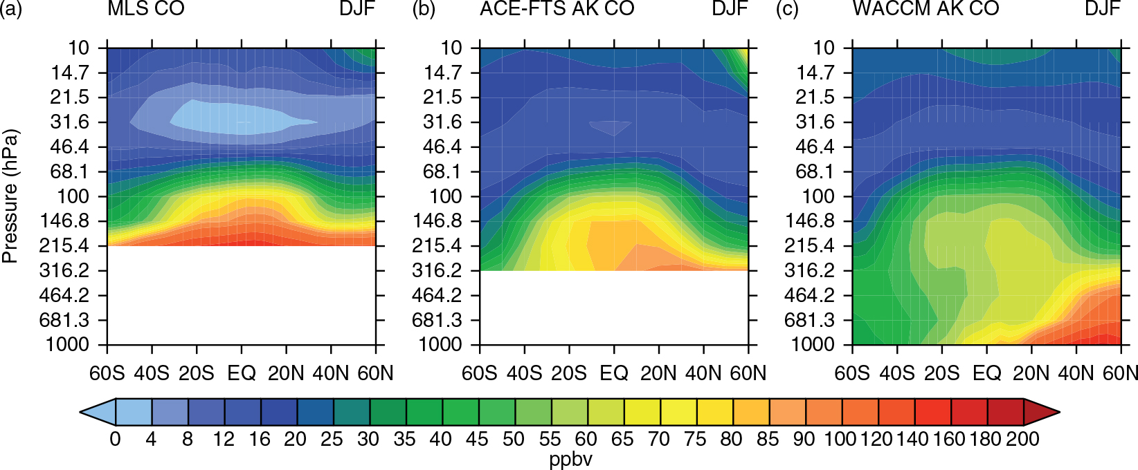
Fig. 2
The latitude–height cross-sections of December–January–February zonal mean CO mixing ratios (unit: ppbv) derived from (a) MLS data, (b) ACE-FTS data and (c) the model simulation in run E0. The ACE-FTS CO and the modelled CO are weighted by the MLS averaging kernels.
Figure 3 shows temporal and vertical variations of the modelled and MLS zonal mean CO anomalies in tropics (10°N–10°S). Figure 3a indicates that the positive MLS CO anomalies in late 2006 and 2010 are larger than those in the other years. The larger CO anomalies in late 2006 and 2010 have been found to be related to the intense fires in Indonesia and South America thought to be affected by ENSO and the phase of the Indian Ocean Dipole, respectively (e.g. Duncan et al., 2007; Field and Shen, 2008; Liu et al., 2013). The sea surface temperatures and sea-ice fractions used in the model simulations are monthly mean values averaged over the time period from 1995 to 2000, and the surface CO emissions used in the model have no inter-annual variations; therefore, the modelled inter-annual variability of CO in the UTLS region is rather small. Note that the QBO signals exist both in the modelled and MLS data above 20 hPa although the QBO signal in MLS CO is slightly weaker and more irregular than that in the modelled CO. The MLS CO data show evident SAO signals between 215 and 146 hPa with two maxima in March–April and October–November and two minima in January and July at these levels, consistent with the results reported in the previous literature (e.g. Schoeberl et al., 2006; Liu et al., 2013). The modelled CO also shows obvious SAO signals in the UTLS, which are in good accordance with the MLS CO. The feature that the negative CO anomalies in the boreal winter and spring at 215 hPa rise up to a lower altitude than the negative anomalies in other months of the same year is also well simulated. Moreover, the AO signals with the positive anomalies in the first half of the year and the negative anomalies in the second of the year above 100 hPa in the MLS CO are also evident in the modelled CO, although the modelled CO anomalies are overall weaker than the corresponding MLS CO anomalies.
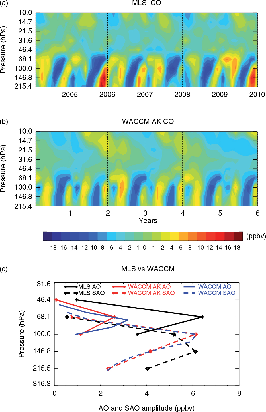
Fig. 3
The (a) MLS and (b) modelled zonal mean CO anomalies in run E0 averaged over the latitude band 10°N–10°S. The modelled CO anomalies are weighted by MLS averaging kernels. The anomalies here are defined as detrended CO time series with 6 yr mean removed from the original time series following Ricaud et al. (2009). Note that only 6 yr of model data are shown since the MLS CO observations cover years from 2005 to 2010. (c) Vertical profiles of the amplitude of the AO (solid lines) and SAO (dashed lines) of zonal mean CO anomalies derived from MLS observations (black lines) and the model simulations (red lines and blue lines). The model results weighted by MLS averaging kernels are shown in red lines. See text for more details of how the AO and SAO amplitudes are estimated.
Figure 3c gives the amplitudes of the AO and SAO signals in the MLS and modelled zonal mean CO anomalies averaged over the latitude band 10°N–10°S. All amplitudes are calculated using the same method as that of Pascoe et al. (2005) in which the amplitude is a function of the ratio of the sum of the squares of the cycle harmonics to the sum of the squares of all harmonics. This ratio is then multiplied by the square root of two times of the standard deviation of the CO anomalies to yield the amplitude. Our analysis indicates that the power of the MLS AO harmonics accounts for 35–80% of CO variability between 100 and 46 hPa with a maximum of 80% at about 68 hPa, while the power of the AO harmonics in the modelled CO (with MLS averaging kernels) accounts for 15–49% of CO variability at these altitudes with a maximum of 49% at about 68 hPa. Comparing the AO amplitudes in the MLS CO with that in the modelled CO, we can see that the AO amplitude in the modelled CO is smaller than that in the MLS data. The maximum amplitude around 68 hPa in the modelled CO is about 2.5 ppbv, less than half of the maximum amplitude in the MLS CO. In terms of SAO, the power of the SAO harmonics accounts for 48–62% of the MLS CO variability between 215 and 100 hPa with a maximum 62% centred at around 147 hPa, and the power of the SAO harmonics accounts for 37–78% of the modelled CO variability between 147 and 100 hPa with a maximum 78% centred at about 100 hPa. The modelled CO without MLS averaging kernels is also shown in Fig. 3. It can be noticed that the maximum amplitude of AO in the modelled CO without weighting by MLS averaging kernels is larger and shifted to lower altitudes (70 hPa) compared with that of the modelled CO weighted by MLS averaging kernels.
Overall, the model can well simulate the observed SAO and AO signals in the MLS CO anomalies, although the low bias exists in the modelled absolute values of CO mixing ratios in the UT (Fig. 2) and slight differences exist in the SAO and AO amplitudes and their vertical variations (Fig. 3) between the observed data and the model simulations.
3.2. Factors influencing CO variations in the UTLS
In this section, we attempt to clarify the relative importance of the various processes in modulating CO variability in the tropical UTLS region. Figure 4 shows temporal and vertical variations of the modelled differences in zonal mean CO anomalies between runs R0 (Total) and R1 (rmEmis), runs R1 (rmEmis) and R2 (rmEmis+rmUb) and runs R2 (Trans+Chem) and R3 (Trans). The zonal mean CO anomalies in runs R0 (Total), R2 (Trans+Chem) and R3 (Trans) are also shown separately.
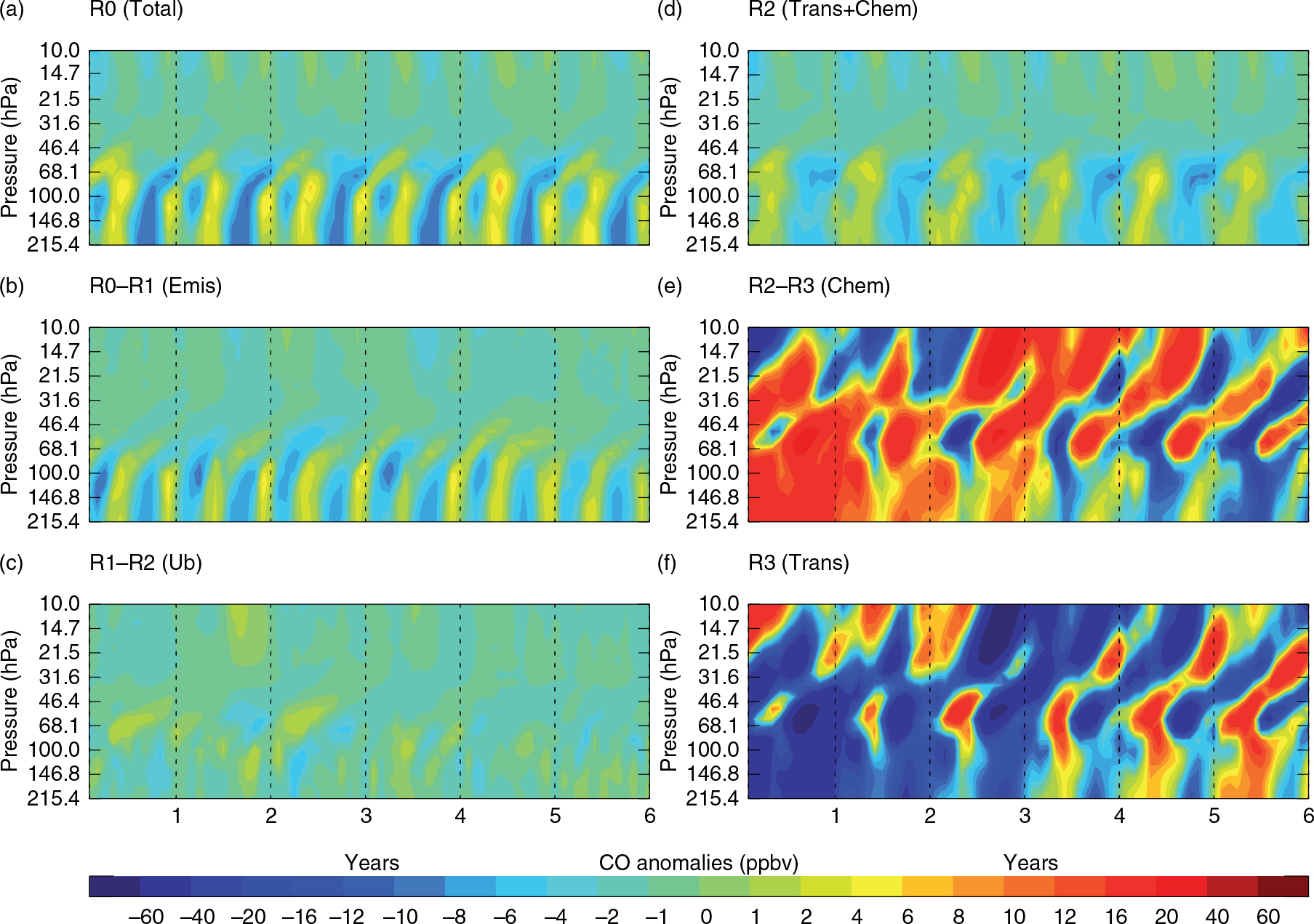
Fig. 4
The modelled zonal mean CO anomalies or difference in CO anomalies averaged over the latitude band 10°N–10°S. (a) The anomalies in run R0 (total), (b) the differences in CO anomalies between run R0 (Total) and run R1 (rmEmis) (i.e. the anomalies caused by the surface emissions), (c) the differences in CO anomalies between run R1 (rmEmis) and run R2 (rmEmis+rmUb) (i.e. the anomalies caused by the CO upper boundary), (d) the anomalies in run R2 (Trans+Chem) (i.e. the anomalies caused by the combination of the chemical and dynamical processes), (e) the differences in CO anomalies between run R2 (Trans+Chem) and run R3 (Trans) (i.e. the anomalies caused by chemical processes) and (f) the anomalies in run R3 (Trans) (i.e. the anomalies caused by dynamical processes).
According to the configuration of R0 (Total), the simulated CO anomalies in run R0 (Total) result from the combined effects of CO surface emissions, CO upper boundary, chemical and dynamical processes on CO variability. The differences in zonal mean CO anomalies between runs R0 (Total) and R1 (rmEmis) shown in Fig. 4b are caused by CO surface emissions with seasonal variations. Figure 4b clearly shows that the SAO signal dominates the CO differences between run R0 (Total) and run R1 (rmEmis) in the UTLS region, confirming that the semi-annual variation of CO surface emissions is the key driver for the semi-annual variation of CO there (Schoeberl et al., 2006). Comparing Fig. 4a with Fig. 4b, we can see that the negative values in February shown in Fig. 4b are smaller than that in Fig. 4a, while the negative values in September–October shown in Fig. 4b are larger than that in Fig. 4a. The differences between Fig. 4a and b suggest that the time variation of CO surface emissions is not the only driver for the CO SAO signal and other processes also play a role in generating it. In addition, the obvious AO signal with the positive anomalies in the first half of the year and negative anomalies in the second half of the year in the LS can be seen in Fig. 4a, but not in Fig. 4b, implying that the AO signal does not result from CO surface emission variations.
The CO differences between runs R1 (rmEmis) and R2 (rmEmis+rmUb) shown in Fig. 4c highlight the influence of the seasonality of the CO upper boundary. It is apparent that the seasonal variation of the CO upper boundary has a rather small impact on the temporal variability of CO in the UTLS region.
The zonal mean CO anomalies in run R2 (Trans+Chem) shown in Fig. 4d result from the combined effects of dynamical and chemical processes. The AO signal in run R2 (Trans+Chem) is in good accordance with that in run R0 (Total) above 85 hPa, confirming that the AO signal of CO in the LS mainly results from the combined effects of dynamical and chemical processes, while CO surface emission variations make no significant contributions to it. However, the AO signal in run R2 (Trans+Chem) is slightly stronger than that in run R0 (Total), suggesting that the semi-annual variations of CO surface emissions tend to weaken the CO AO signals. There also exists a weak SAO signal in Fig. 4d with the maximum magnitude at 100 hPa, and this SAO signal is synchronized with that in run R0 (Total). It is apparent that dynamical and chemical processes together can also generate a weak SAO signal in CO, although the dominating driver of SAO signal in CO is the seasonality of CO surface emissions. The differences in CO anomalies between runs R2 (Trans+Chem) and R3 (Trans) shown in Fig. 4e represent the effect of chemical processes on CO temporal variations, while the anomalies in run R3 (Trans) shown in Fig. 4f result from dynamical processes only. It is evident that the anomalies shown in Fig. 4e approximately mirror the anomalies shown in Fig. 4f, suggesting that dynamical and chemical processes have the opposite effects on the variability of CO in the UTLS region. This CO variation in the LS has also been reported by Abalos et al. (2012, 2013). Moreover, our analysis indicates that this feature also exists in the UT and near the tropopause. The dynamically induced CO anomalies in Fig. 4f are approximately in phase with the CO anomalies in Fig. 4d. Therefore, dynamical processes control the phase of CO variability in the UTLS region, while chemical processes tend to weaken the amplitude of CO variability since the chemically induced CO anomalies are out of phase with the dynamically-induced CO anomalies.
Note that the modelled CO tape recorder signals in run R0 (Total) only rise up to about 40 hPa, whereas the observed tape recorder signals of other gases such as H2O, CO2 and HCN rise up to 10 hPa (Mote et al., 1995; Andrews et al., 1999; Pumphrey et al., 2008). In run R3 (Trans), the chemical reactions associated with CO are switched off, and the AO signal of CO in the LS can also rise up to 10 hPa. This suggests that chemical processes have a significant impact on the altitude extent of CO AO signals. The 11–13 months band-pass filtered anomalies in run R3 (Trans) (not shown) provide more clear evidence that the AO signal of CO in run R3 (Trans) can rise slowly up to 10 hPa, along with a phase shift in the stratosphere with height.
Figure 5 shows amplitudes of CO annual cycle and semi-annual cycle at different levels in different runs and their differences between different runs. The differences in AO amplitudes between runs R1 (rmEmis) and R2 (rmEmis+rmUb) are close to zero, further confirming that the seasonality of the CO upper boundary has no significant effect on the CO annual cycle. The vertical variations of CO AO amplitudes in run R2 (Trans+Chem) are nearly identical to those in R0 (Total), consistent with the result in Fig. 4 that the CO annual cycle between 100 and 46 hPa is primarily caused by dynamical and chemical processes together. Note that between 100 and 46 hPa, the amplitude of CO AO in run R2 (Trans+Chem) is around ~1 ppbv larger than that in run R0 (Total), implying that the effect of CO surface emissions tends to weaken the amplitude of the CO annual cycle in the UTLS in the order of 1 ppbv. In accordance with Fig. 4, the CO AO amplitude in run R3 (Trans) is much larger than that in run R0 (Total), that is, the AO signal in the modelled CO largely results from dynamical processes while the chemical processes tend to weaken CO AO signals.
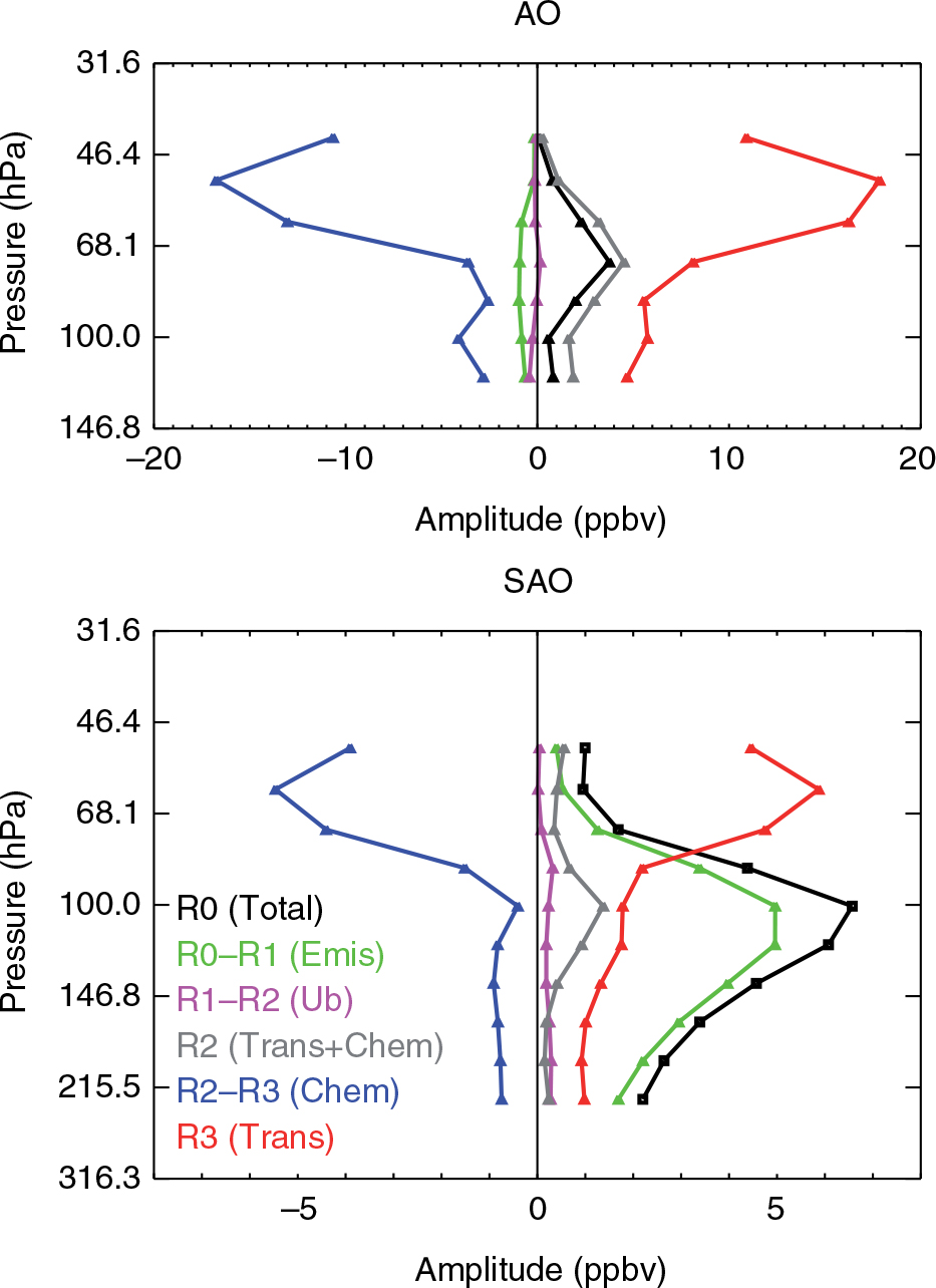
Fig. 5
Vertical profiles of the amplitude of the AO (top) and SAO (bottom) of zonal mean CO anomalies in different runs and their difference between different runs. Black, grey and red lines represent the amplitudes in run R0 (Total), run R2 (Trans+Chem) and run R3 (Trans), respectively. Green, purple and blue lines represent the difference between run R0 (Total) and run R1 (rmEmis), between run R1 (rmEmis) and run R2 (rmEmis+rmUb), and between run R2 (Trans+Chem) and run R3 (Trans), respectively.
The CO SAO amplitudes in the run R2 (Trans+Chem) are much smaller than that in run R0 (Total) while the difference in SAO amplitude between runs R0 (Total) and R1 (rmEmis) is very similar to the CO SAO amplitude in run R0 (Total). This result suggests that the seasonal variations of CO surface emissions make the largest contributions to the CO SAO signal in the tropical UTLS region. The small but positive CO SAO amplitude in run R2 (Trans+Chem) implies that the net effect of dynamical and chemical processes on CO SAO signals is to enhance their amplitudes. The above analysis reveals that the seasonality of CO surface emissions explains most of the CO SAO signal, with the remainder due to dynamical and chemical processes. In terms of the maximum SAO amplitude of ~6.5 ppbv in run R0 (Total) at 100 hPa, the seasonality of CO surface emissions contributes to 5 ppbv.
From Figs. 4 and 5, we can see that dynamical and chemical processes as well as the seasonal variations of CO surface emissions all have an impact on the CO AO and SAO signals in the tropical UTLS region. However, their impacts are different at different altitudes, and their relative importance in generating CO AO are also different from that in generating CO SAO. In the following, we attempt to further clarify which dynamical and chemical processes are mainly responsible for the CO AO and SAO signals in tropical UTLS region.
3.3. Chemical and dynamical processes influencing CO variations in the UTLS
Figure 6 shows the seasonal variations of the monthly mean tropical CO anomalies at different altitudes associated with chemical production, chemical loss and net chemical effects. The seasonal variations of the CO anomalies in run R3 (Trans), the OLR and vertical component of the BD circulation averaged over 10°N–10°S are also shown in Fig. 6. It is apparent that both the chemical production and loss of CO in the UTLS have an evident seasonal variation. The variation of the CO anomalies due to chemical processes is in phase with and on the same order of the CO anomalies caused by chemical loss in the UT (Fig. 6c) and near the tropopause (Fig. 6b), suggesting that the CO chemical loss dominates the seasonality of the CO variations associated with chemical processes. In the LS (Fig. 6a), the chemical production becomes important in affecting the seasonality of the CO anomalies, but the chemical production is still much smaller in magnitude than the chemical loss of CO. In accordance with Fig. 4, the seasonal variation of the CO anomalies in run R3 (Trans) is out of phase with the seasonal variation of the CO anomalies caused by the net chemical effects. The magnitude of dynamically induced CO anomalies is slightly larger than that of chemically induced CO anomalies.
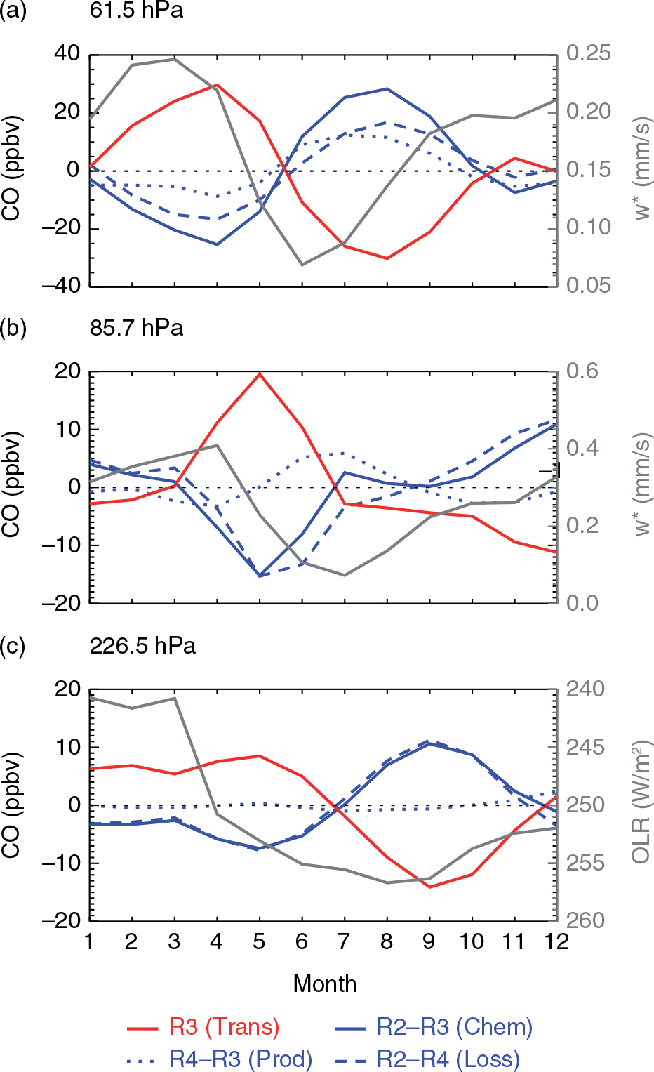
Fig. 6
Seasonal variations of the differences in modelled zonal mean CO anomalies averaged over the latitude band 10°N–10°S between different runs at (a) 61.5 hPa, (b) 85.7 hPa and (c) 226.5 hPa. Blue solid lines, blue dotted lines and blue dashed lines represent the differences between runs R2 (Trans+Chem) and R3 (Trans) (i.e. the CO changes associated with the chemical processes), R4 (Trans+Prod) and R3 (Trans) (i.e. the CO changes associated with the CO chemical production), and runs R2 (Trans+Chem) and R4 (Trans+Prod) (i.e. the CO changes associated with the CO chemical loss). Red solid lines represent the CO anomalies in runs R3 (Trans) (i.e. the CO changes associated with dynamical processes). The time series of the zonal mean OLR averaged over 10°N–10°S (grey solid line) is also shown in Fig. 5c. The time series of residual vertical velocities (grey solid line) at 61.5 and 85.7 hPa are also shown in Fig. 6a and b, respectively.
To understand what dynamical processes generate seasonal variation of CO in the tropical UTLS region, the seasonal variation of the OLR averaged over 10°N–10°S is examined in Fig. 6c. Figure 6c indicates that the tropical OLR in boreal winter and spring is lower than that in boreal summer and autumn, that is, convective activities in boreal winter and spring are stronger than that in summer and autumn. It is known that tropical deep convection has a significant impact on tracer distributions in the UTLS region (e.g. Duncan et al., 2007; Liu et al., 2007, 2013; Li et al., 2014). The seasonal variation of the tropical convective activities shown in Fig. 6c looks overall in phase with the seasonal variation of the modelled CO anomalies associated with dynamical processes, that is, weak convective activities (larger OLR) in July–December correspond to negative CO anomalies at 226.5 hPa. However, Fig. 6c indicates that tropical convective activities are strongest in boreal winter but the maximum dynamically induced CO anomalies in the UT (226.5 hPa) occur in May. This mismatch in the times that the maximum CO anomalies and the strong convective activities appear (shown in Fig. 6c) suggests that the upward transport of CO surface emissions by convection is not the only dynamical process controlling CO seasonal variations in the tropical UT. Moreover, the CO maximum in May can also be seen near the tropical tropopause (85.7 hPa), and the CO maximum at 85.7 hPa is larger than that at 226.5 hPa, possibly due to the horizontal transport of CO from the extra-tropics to the tropics in the UT and near the tropopause.
To further understand the influences of dynamical processes on CO variations in the UT and near the tropopause, the horizontal distributions of the modelled CO anomalies and horizontal winds in run R3 (Trans) in May–August at 85.7 hPa are shown in Fig. 7. The horizontal distributions of the MLS CO anomalies and horizontal winds from ERA-Interim data at 100 hPa in May–August are also shown in Fig. 7 for comparison. Note that the MLS CO anomalies are smaller in magnitude than the modelled CO anomalies in run R3 (Trans) as the chemical reactions associated with CO are switched off in run R3 (Trans), and the chemical destruction/production of CO is not present. It is apparent from the ERA-Interim wind fields that the Asian summer monsoon anticyclone in May is close to the equator, and then the anticyclone moves northward from June to August. Accordingly, the centre of the maximum anomaly of the MLS CO inside the anticyclone moves northward. This feature can also be seen in the modelled CO anomalies and horizontal wind fields at 85.7 hPa in run R3 (Trans), suggesting that the model can well capture the monthly evolution of CO along with the onset of the Asian monsoon.
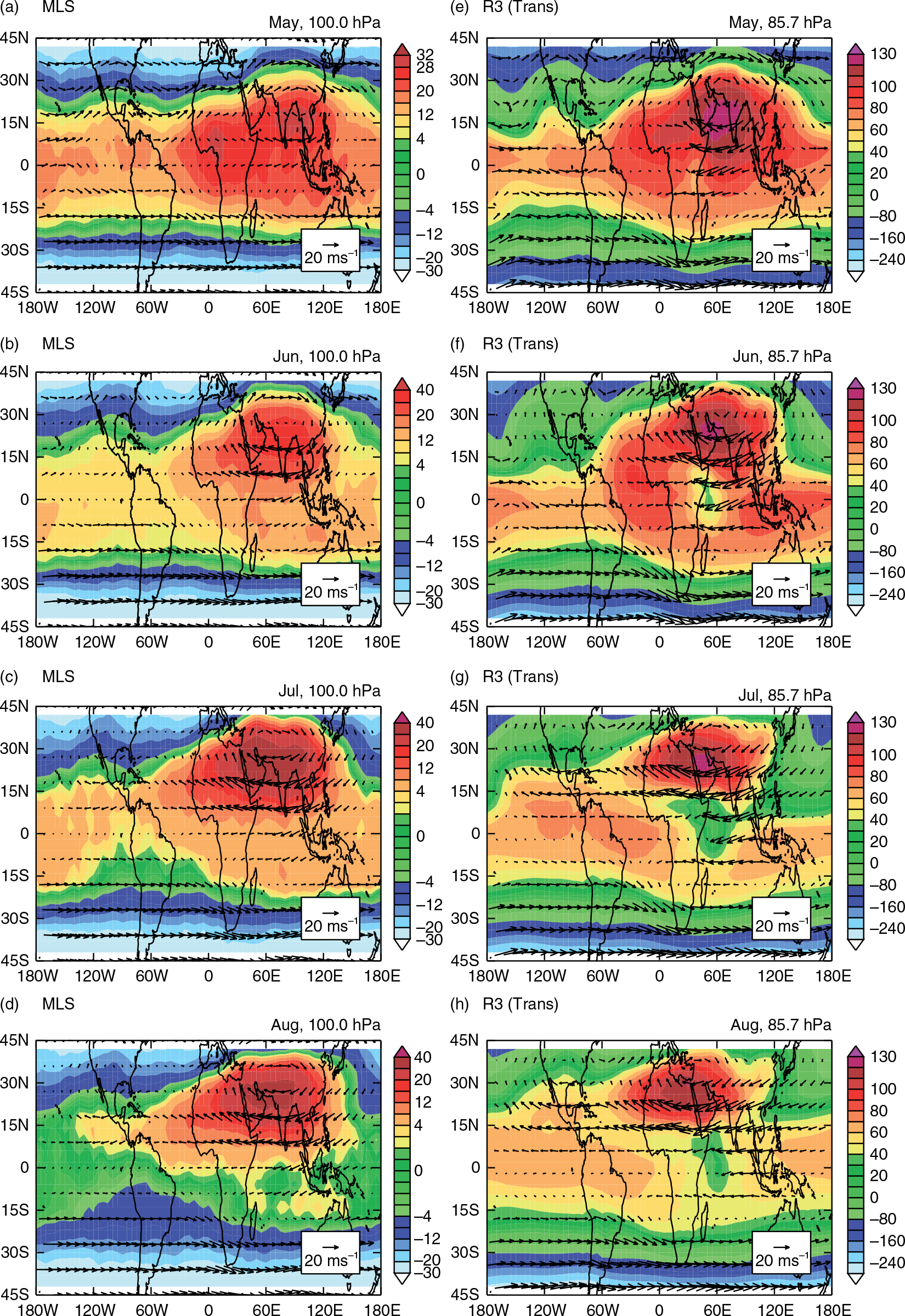
Fig. 7
The horizontal distributions of the monthly mean CO anomalies (deviations from zonal mean CO mixing ratios over the latitude band 42°N–42°S, unit: ppbv) (filled contours) in (a, e) May, (b, f) June, (c, g) July and (d, h) August at (a–d) 100 hPa derived from the MLS CO data and (e–h) 85.7 hPa in the modelled CO in run R3 (Trans). Arrows indicate horizontal wind fields obtained from (a–d) ERA-interim data and (b–h) the model simulations in run R3 (Trans) at the corresponding level.
In May, the southern boundary of the high CO region at 85.7 hPa covers the tropics (10°S–10°N) along the longitude band 0°–100°E with the centre of the CO maximum located at around 15°N (Fig. 7e). Subsequently, with the development of the Asian summer monsoon, the southern boundary of the high CO region moves northward gradually and the centre of the CO maximum reaches to about 30°N in August (Fig. 7f–h). Tao and Chen (1987) pointed out that the onset of the Asian summer monsoon first occurs over the Bay of Bengal and the South China in May. Therefore, the high tropical CO values at 85.7 hPa in May are due to vertical transport of the CO surface emissions over Southeast Asia by the South Asian summer monsoon circulation (Fig. 7e). The tagged CO simulations from biomass burning in Southeast Asia in Duncan et al. (2007) also showed that the emissions from Southeast Asia can increase the tropical CO concentrations in April–June. With the further development of the Asian summer monsoon from June to August, the Asian summer monsoon anticyclone intensifies and its centre moves northward, accordingly, the southern boundary of the high CO region moves northward and the high CO in the anticyclone over Southeast Asia is confined within it (Fig. 7f–h; e.g. Randel and Park, 2006; Park et al., 2007, 2008, 2009; Randel et al., 2010; Bian et al., 2011; Li et al., 2014). Meanwhile, the horizontal transport from the extratropics to the tropics through the eastern flanks of the Asian summer monsoon anticyclone causes a decrease in CO to the south of the anticyclone over the tropics, consistent with the results in previous studies (e.g. Konopka et al., 2009, 2010; Ploeger et al., 2012; Abalos et al., 2013). Consequently, the tropical CO values in the tropical UTLS decrease in the boreal summer.
It is known that the vertical transport of CO is closely linked with the ascending branch of Brewer–Dobson circulation in the tropical LS (e.g. Randel et al., 2007; Schoeberl et al., 2008; Abalos et al., 2012, 2013). Figure 6a indicates that the seasonal variation of CO anomalies at 61.5 hPa in run R3 (Trans) is correlated, with ~1 month time lag, well with the seasonal variation of the vertical velocity of the BD circulation and this time lag approximates the vertical transport time used by the BD circulation to bring tracers at 100–61.5 hPa. It can also be noted from Fig. 6a and b that the magnitude of CO anomalies at 61.5 hPa is larger than that at 100.5 hPa. The above fact is consistent with the result of Schoeberl et al. (2008) that the CO annual cycle between 18 and 20 km reflects the seasonality in the tropical upwelling.
Without considering CO chemical source and sink terms, the annual variation of CO in the LS driven by the BD circulation can be written as (Schoeberl et al., 2008)
here, the overbars represent zonal means, µ is the CO mixing ratio, t is the time, z is the log-pressure height, and are the zonal residual meridional and vertical velocities; the variables with are time averaged and have no AO signals; the AO subscripted variables are the detrended anomalies with 11–13 months band-pass filtered. The terms and reflect the contribution of the vertical and meridional advection to CO AO tendency () associated with the AO signals in and only, as there is no AO signals in , respectively. The terms and reflect the contribution of the vertical and meridional advection to CO AO tendency associated with the pre-existing AO signals in CO, since there are no AO signals in and . In the above equation, the unresolved eddy transport and uncertainties for the resolved terms is represented by ‘Residual’ term.
Figure 8a–c gives the time–height cross-section of , and estimated from the modelled CO anomalies (averaged over the latitude band 10°N–10°S) in run R3 (Trans). A comparison between Fig. 8a and c reveals the relative large CO AO amplitude between 70 and 50 hPa results from the effect of the annual variations in the BD circulation acting on the background vertical gradient in zonal mean CO values, consistent with the results in Schoeberl et al. (2008). The CO tape recorder signals are observed above 50 hPa in Fig. 8a and b, where there is a constant phase shift with altitude, suggesting that the tape recorder signal primarily results from the annual variations of trace gases near the tropopause, which are simply carried upward by the mean field.
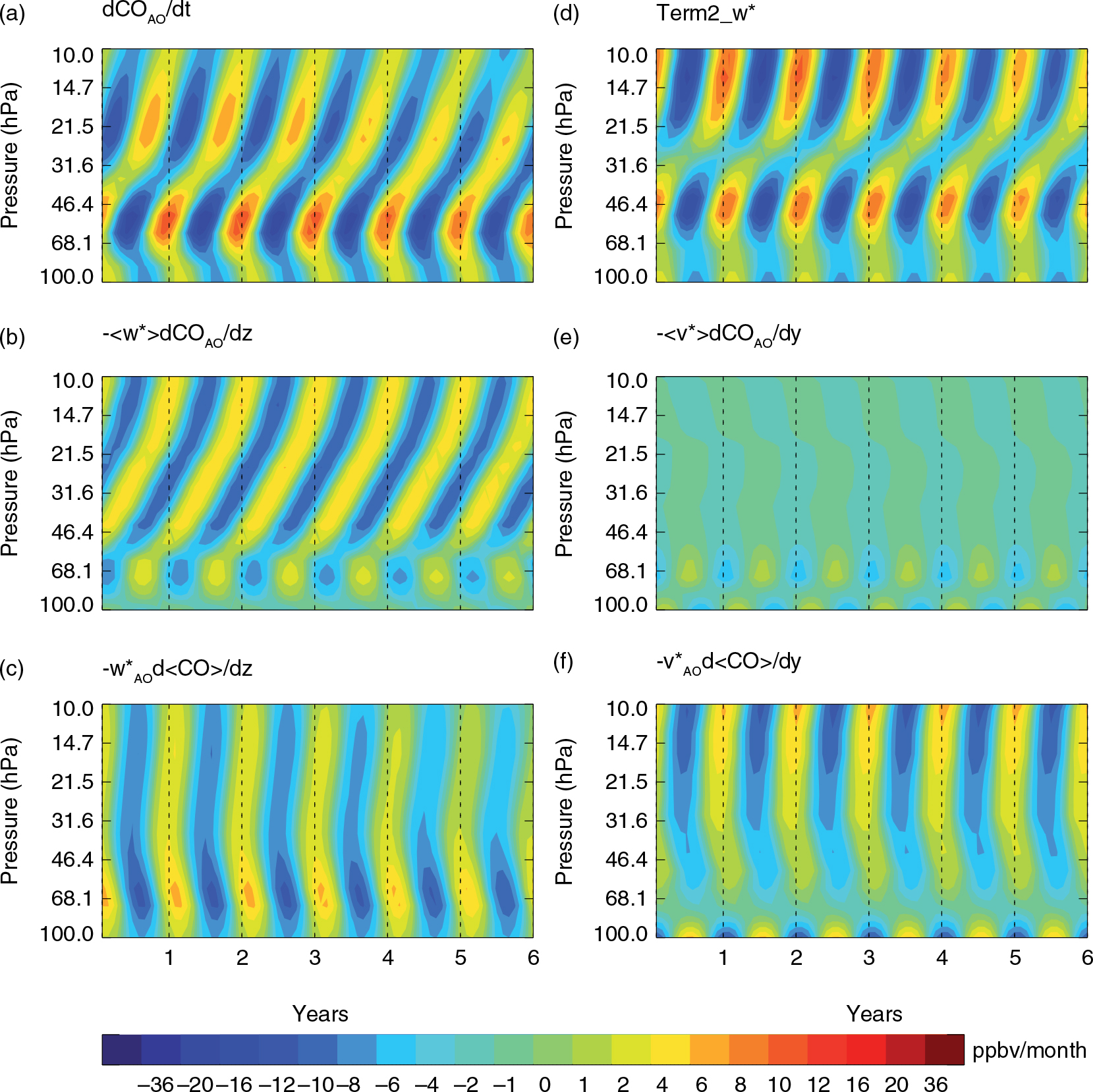
Fig. 8
The time–height cross sections of (a) , (b) , (c) , (d) Term2_w*, (e) and (f) averaged over the latitude band 10°N–10°S derived from the model outputs in run R3 (Trans) (see text for the definitions of these terms).
An interesting feature in Fig. 8c is that acting on the mean <CO> field without seasonal variations tends to generate a seemingly downward propagating signal between 40 and 70 hPa. From Fig. 6a and b, we can see that the seasonal variation of the residual vertical velocities at 61.5 hPa is ~1 month ahead of that at 85.7 hPa. This downward propagating signal of CO is possibly generated by the phase shift with height in the seasonal variations of the vertical component of the BD circulation at these levels. The seasonal variations of the modelled vertical component of the BD circulation averaged over the latitude band 10°N–10°S in run R3 (Trans) also exhibit a ‘downward propagation’ of the minimum between 40 and 70 hPa, particularly in Spring and Summer months (not shown).
Figure 8d gives the time–height cross-section of the sum of two vertical advection terms and (termed ‘Term2_w*’). Note that both the magnitude and the phase of the variations of ‘Term2_w*’ are in good agreement with that of the CO AO tendency shown in Fig. 8a. This result confirms that CO annual variations caused by the BD circulation are primarily driven by vertical advection. Randel et al. (2007) pointed out that it is the annual cycle of tropical upwelling that leads to the annual cycle of CO in the LS. Schoeberl et al. (2008) argued that the CO annual cycle between 18 and 20 km reflects the seasonality of tropical upwelling, and above 20 km it is the annual cycle of CO that is transported upward by the mean upwelling circulation without seasonal variations. Fig. 8d indicates that the CO annual cycle in the LS has a mixed behaviour with the annual variations of tropical upwelling reflected in CO between ~70 and ~50 hPa and a standard tape-recorder signal above 50 hPa, in good agreement with Schoeberl et al. (2008). However, the magnitude of CO tendency above 30 hPa is smaller than that of the ‘Term2_w*’ term, suggesting that vertical advection is not the only dynamical process controlling the CO variations in the middle stratosphere, and there should be other dynamical processes which tend to weaken the amplitude of CO AO signal above 30 hPa. The effect of the horizontal advection by the BD circulation on the temporal and vertical variations of CO AO tendency in the tropical stratosphere can be inferred from the two terms: and . Figure 8e and f shows the temporal and vertical variations of these two terms. We can see that the magnitude of term is rather small and has no significant effect on the variations CO AO tendency (Fig. 8e). Figure 8f indicates that the effect of the meridional advection of the BD circulation on variations of CO in the tropical stratosphere is dominated by the annual variations in the meridional components of BD circulation. The net effect of the meridional advection of CO by the BD circulation tends to amplify the amplitude of the CO AO signal above 30 hPa. That is to say, the dynamical processes which tend to weaken the amplitude of CO AO signal above 30 hPa is not meridional advection of CO by the BD circulation and may be due to eddy transport included in the ‘Residual’ term that we haven't discussed.
4. Summary and conclusions
The WACCM is used to investigate the impacts of the CO surface emissions, the CO upper boundary, dynamical and chemical processes on the temporal variations of CO in the tropical UTLS region. Our simulations show that CO semi-annual signals in the tropical UTLS region are primarily driven by the semi-annual variations of the tropical biomass burning emissions, and the contribution of dynamical and chemical processes to the CO semi-annual signals is small. In terms of the CO SAO amplitude at 100 hPa, the variations of CO surface emissions account for ~80% of the maximum amplitude, while the combined effects of dynamical and chemical processes account for no more than 20%. The CO annual cycle in the LS is mainly driven by the dynamical and chemical processes together, while the variations in CO surface emissions tend to weaken the amplitude of the CO annual cycle about 1 ppbv. The seasonality of CO upper boundary has no significant impact on the CO variability in the tropical UTLS.
The seasonality of chemical processes associated with CO is dominated by the variations of the chemical CO loss in the UT and near the tropopause. The variations of the CO chemical production are rather small in the tropical UT but become important in affecting the seasonality of CO in the LS above 86 hPa. It is interesting that the AO signal in the LS can rise slowly up to 10 hPa with a phase shift with height, the level of the tape recorder signal of other gases such as H2O, CO2 and HCN rises up to, in the simulations without chemical processes, verifying that the CO tape recorder signal fades out at about 40 hPa is indeed due to the CO chemical processes. Based on tracer budgets analysis using transformed Eulerian mean formalism, Abalos et al. (2012) found that the chemical processes associated with CO are out of phase with CO seasonal variations generated by dynamical processes in the LS. Our analysis confirms their results. Our analysis further reveals that this feature also exists in the UT and near the tropopause. Moreover, our simulations indicate that the magnitude of dynamically induced CO anomalies is slightly larger than that of chemically induced CO anomalies.
The seasonal variations in tropical convective activities, the in-mixing driven by the Asian summer anticyclonic circulation and the BD circulation all make a contribution to CO variability in the tropical UTLS. The relatively strong convection in December–May and weak convection in other months in tropics would lead to high CO in the boreal winter and spring and low CO in the boreal summer and fall in the tropical UT and near the tropopause. The effects of the in-mixing on the tropical CO are different in different months. The high tropical CO values at 85.7 hPa in boreal late spring and early summer are due to vertical transport of the CO surface emissions over Southeast Asia by the South Asian summer monsoon circulation over the Bay of Bengal and the South China. The in-mixing process through the eastern flanks of the well-known Asian summer monsoon anticyclone in the boreal summer (e.g. Randel and Park, 2006; Park et al., 2007, 2008 2009; Randel et al., 2010) causes a decrease in the tropical CO, consistent with the results in previous studies (e.g. Konopka et al., 2009, 2010; Ploeger et al., 2012; Abalos et al., 2013). The joint effects of the deep convection and the horizontal transport of CO from the extratropics into the tropics lead to relatively large CO mixing ratios in the boreal late spring and early summer in the tropical UT and near the tropopause.
Our simulations also confirm that the CO annual cycle reflects the seasonality of the tropical upwelling between ~70 and ~50 hPa, and above 50 hPa is simply transported upward by the mean upwelling circulation without seasonal variations (i.e. a standard tape-recorder signal), in good agreement with Schoeberl et al. (2008). In addition, our analysis also reveals that the annual variations in the meridional components of the BD circulation can amplify the annual fluctuations of CO above 30 hPa.
5. Acknowledgements
This work was supported by the National Science Foundation of China (41175042) and the National Science Foundation of China (41225018). We thank the NOAA for providing the OLR data. We also thank the ECMWF for providing the reanalysis data. MLS CO data were downloaded from NASA's Goddard Space Flight Center and processed following recommendation from Livesey et al. (2007). The ACE mission is funded primarily by the Canadian Space Agency. Computing support is provided by the Gansu Computing Center. We also thank the two anonymous reviewers and the editor for their helpful comments and suggestions.