
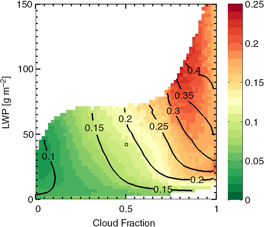
Fig. 1
Average albedo (black contours) and standard deviation of albedo (colours) as a function f c and LWP. The plot only shows data points where the frequency of occurrence is higher than 0.01%. The black square represents a grid point at f c =0.5 and LWP=40 g m−2 which is further analysed as an example in Fig. 2.
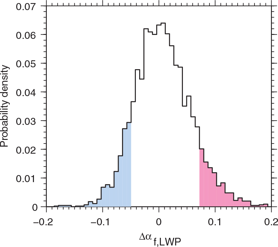
Fig. 2
Probability density function of albedo perturbations, , at f c =0.5 and LWP=40 g m−2, that is, all albedo perturbations in the black square of Fig. 1. The blue- and pink-shaded regions represent parts of the PDF below and above the 10th and 90th percentiles, respectively.
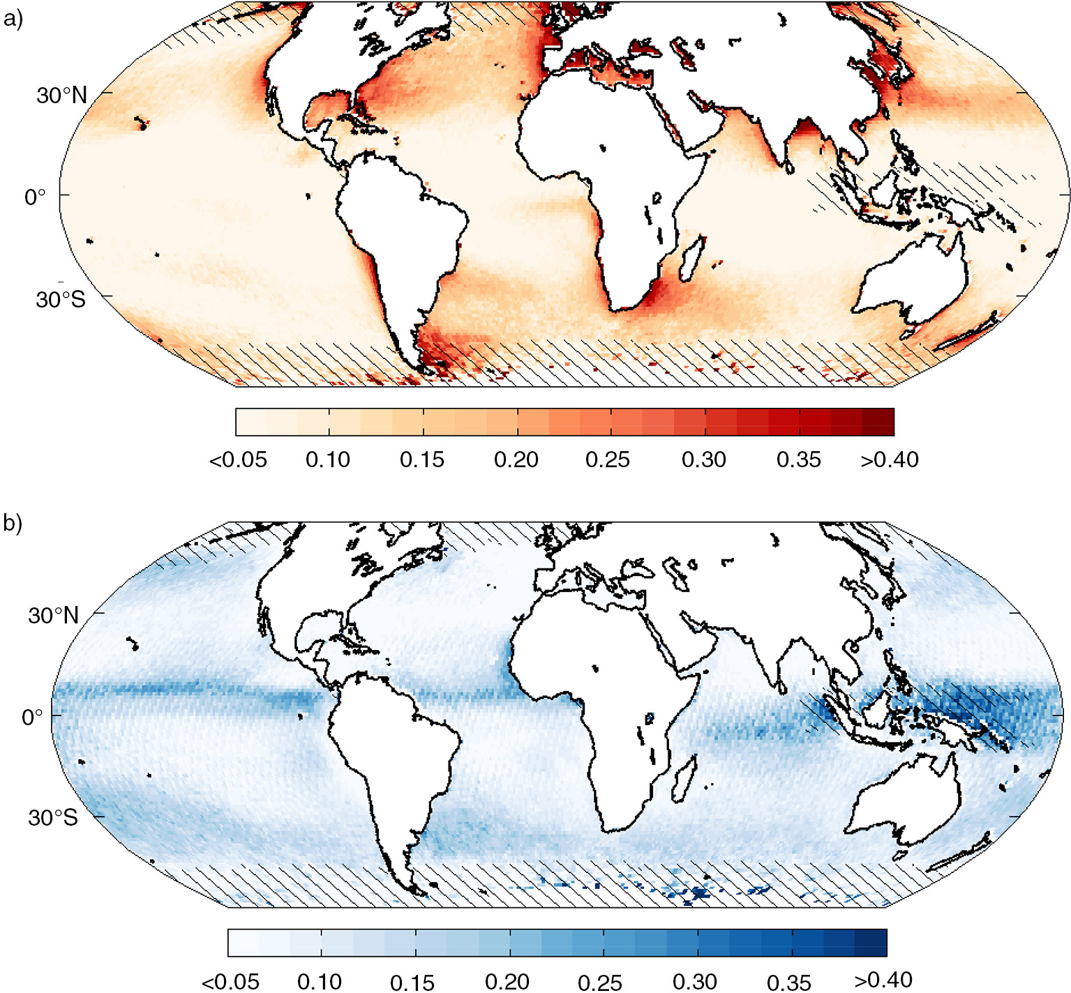
Fig. 3
(a) The fraction of days for each 1°×1° grid point over the global ocean for which the albedo perturbation is above the 90th percentile in each PDF of . The fraction is obtained by applying G to each such perturbed value of to obtain a subset of -values at every 1°×1° grid point and dividing by the total number of -values at that same location. An example of a PDF of for one pair of f c and LWP values is shown in Fig. 2. (b) Same as in (a) but for the 10th percentile of the albedo perturbations. Hatched areas represent regions where the number of successful retrievals are less than 10% of the maximum number of available retrievals for each 1°×1° grid cell.
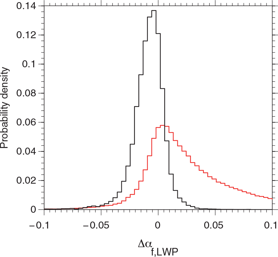
Fig. 4
Probability density function of values of which were sampled in regions with a frequency value above 0.3 in Fig. 3a (red line) and Fig. 3b (black line).
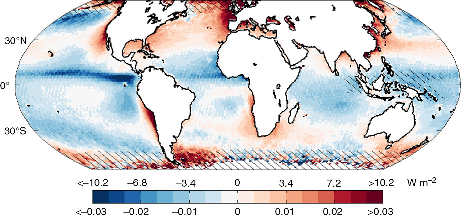
Fig. 5
The integral of Δα independent of f c and LWP at each 1°×1° grid cell over global ocean. The colours also represent the resulting radiative perturbations in W m−2 obtained by multiplying the albedo perturbations by the mean solar insolation of 340 W m−2. Hatched areas represent regions where the number of successful retrievals are less than 10% of the maximum number of available retrievals for each 1°×1° grid cell. The spatial detection limit of 0.003, that is, the difference between each value of the colour bar, is based on the global mean minimum difference between each 1°×1° grid point and its eight neighbouring grid points.
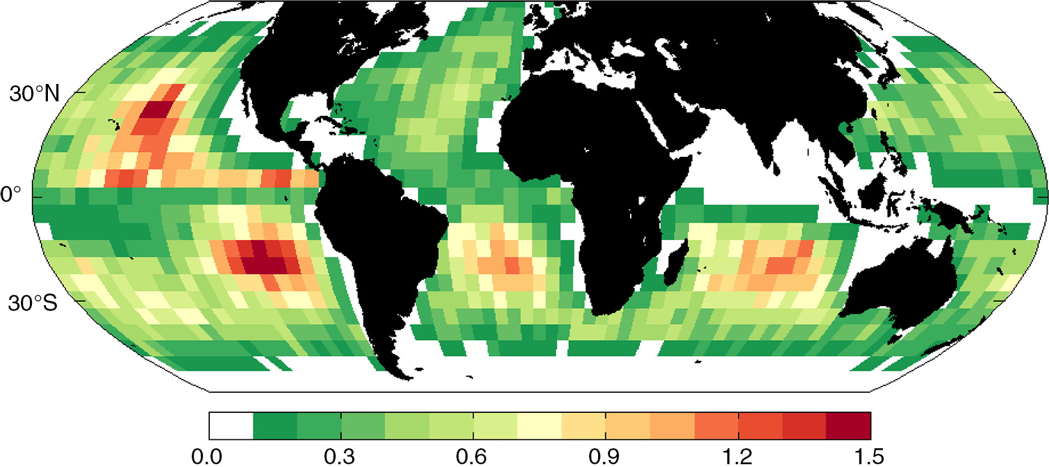
Fig. 6
Mean precipitation rate (mm day−1) at cloud base from warm low-level liquid clouds (cloud top height <3 km and cloud top temperature >273 K as determined by MODIS) estimated with space-borne radar measurements from CloudSat (Lebsock and L'Ecuyer, 2011). The data shown are identical to what was shown in Fig. 5 of Wood et al. (2012) except that all ocean regions are shown, and not only regions dominated by extensive low clouds in the subsidence regions. Regions with high precipitation (red) generally coincide with the blue areas of Fig. 5, suggesting the importance of considering aerosol sinks along with sources when interpreting the map of albedo perturbations.