Geographically coherent patterns of albedo enhancement and suppression associated with aerosol sources and sinks

1. Introduction

Identifying and quantifying the factors that govern the Earth's albedo are essential for understanding the amount of solar energy available to the system. The albedo depends on several key variables: surface properties, clear-sky reflection of sunlight by aerosols, and most importantly, the fractional coverage and optical properties of clouds. Using a simple approximation, the total albedo can be expressed as a linear function of its cloudy and clear-sky components and the fractional cloud cover (Cess, 1976). The fractional cloud cover has been shown to be well correlated with the albedo of synoptic-scale scenes in key marine locations and can explain a dominant fraction of the variance in total albedo (Loeb et al., 2007; Bender et al., 2011; Engström et al., 2014). When the fractional cloud cover variability is taken into account, the remaining variability depends on the clear-sky albedo and on the albedo of clouds, of which the latter is to a large extent dependent upon the total amount of condensed water, and to a smaller extent, the cloud droplet number concentration (George and Wood, 2010). From a climate change perspective, the variability in the cloud droplet number concentration is of specific interest because an increased concentration of aerosol particles is expected to lead to an increase in the cloud droplet number concentration, and subsequently in cloud albedo through the first aerosol indirect effect (Twomey, 1974, 1977). Thus, observations of albedo hold important information about both clear-sky scattering of aerosols and aerosol impacts on cloud albedo.

A number of studies have used the simplified relationship between albedo and cloud fraction from Cess (1976) to attempt to isolate and study aerosol effects on albedo in both observations and models (Lebsock et al., 2008; Quaas et al., 2008; George and Wood, 2010; Chen et al., 2014; Engström et al., 2014). However, the presence of multiple albedo controlling factors makes it difficult to isolate aerosol-induced changes in albedo using observations (Stevens and Brenguier, 2009), and it is even more difficult to estimate the anthropogenic component of such changes. Current estimates of the total aerosol anthropogenic forcing, which includes direct scattering and absorption of sunlight by aerosols as well as indirect aerosol effects on cloud macro- and microphysical properties (Twomey, 1974; Albrecht, 1989) and associated fast feedback processes, range from −1.9 to −0.1 W m⁻² and currently constitute the greatest source of uncertainty in the anthropogenic forcing of climate (IPCC, 2013). The global perturbation in albedo that would correspond to a forcing of −1.9 W m⁻² amounts to only 0.006, a tiny quantity which is difficult to detect and measure using today's satellite instruments (Seidel et al., 2014). Nonetheless, the negative forcing of aerosols could, in the present-day climate, potentially balance a significant fraction of the positive forcing due to anthropogenic greenhouse gases, which range between 2.3 and 3.4 W m⁻² (IPCC, 2013), and thus its magnitude strongly affects the current empirical estimates of climate sensitivity (see e.g. Kiehl, 2007).

Here, we introduce a method by which we examine the spatial distribution of the albedo variability of clear-sky and liquid-cloud scenes independent of variations in the two dominant factors of albedo: cloud fraction and liquid water path (LWP). The motivation for constraining variability in these two quantities is that the remaining variability in albedo will be, to a large extent, dependent on clear-sky scattering by aerosols and on differences in cloud optical properties related to the cloud droplet number concentration, and thus on the atmospheric aerosol particle population. To reduce the influence of varying surface albedos, we focus on global ocean areas between 60° S and 60° N.

The question in focus is whether there is a geographically coherent pattern related to variations in albedo that cannot be explained by variations in cloud fraction and LWP. We start by illustrating the ways in which cloud fraction and LWP control the total albedo and continue to examine the geographical structure of extreme albedo perturbations constrained by narrow limits in cloud fraction and LWP. We then continue to quantify the magnitude of such albedo perturbations and discuss the implications and radiative effects of the observed geographical structure.

2. Data and methods

We analyse all-sky albedo (α) as obtained from satellite-observed radiometric fluxes from CERES (Clouds and the Earths Radiant Energy System) (SSF1-deg Edition 2.7, Wielicki et al., 1996) and its dependence on cloud fraction (f _c) and LWP derived from MODIS (MODerate resolution Imaging Spectroradiometer) (Version 6, King et al., 2003). Both instruments are carried by Aqua, a sun-synchronous polar orbiting satellite that crosses the equator at 13:30 local time in ascending node and distributed as part of the Single Satellite Footprint (SSF) collection. Daily overpass data are obtained for the period between July 2002 and June 2014 and aggregated to a 1°×1° degree resolution. To minimise the effect of differences in albedo because of varying surface properties, we perform the study over the global ocean between 60° S and 60° N. Higher latitudes are avoided because of the presence of highly reflective sea-ice. To further simplify the interpretation of the data, we focus on scenes which are either determined as clear-sky or found to consist only of liquid clouds. In the latter case, we only consider retrievals where (1) a LWP was successfully retrieved, (2) the cloud top temperature was above 273 K and (3) no ice-phase water was detected by the retrieval algorithm. This represents 20 million retrievals over ocean or about 23% of the total amount of data available over ocean for the period of study.

The method of analysis makes use of the empirically observed relationship between albedo, f _c and LWP. The complete set of retrieved values of albedo is sorted based on the co-retrieved value of f _c and LWP into equally spaced bins, where the bin widths are set to Δf _c =0.01 and ΔLWP=1 g m⁻². The procedure yields a range of α values at every grid point in f _c-LWP-space. We refer to this procedure of binning albedo from geographical space to f _c-LWP-space as applying the binning operator L so that $\mathbf{L}{\alpha }_{i,j}^n={\alpha }_{f_c,\text{LWP}}^n$, where i,j denotes the index of a 1° longitude and latitude point over global ocean, and n is the time-index representing each day. The purpose of the operator L is to isolate the variability in albedo, which is due to varying cloud optical properties and clear-sky scattering of aerosols and is not caused by varying f _c and LWP. To move albedo values back from f _c-LWP-space to geographical space, while still keeping the time-dimension, we define another operator G, so that $\mathbf{G}{\alpha }_{f_c,\text{LWP}}^n={\alpha }_{i,j}^n$. Essentially, G reverses the binning procedure back to the corresponding i,j-index.

We note that the analysis does not filter out the effect of varying solar zenith angles (Grosvenor and Wood, 2014), or other albedo influencing factors, e.g. related to a heterogeneous in-cloud distribution of condensate (Rossow et al., 2002). We also note that, for an assumed plane-parallel liquid cloud, the cloud albedo is highly sensitive to small differences in LWP when the absolute value of LWP is low (Wood, 2012). This will mainly cause large differences in the all-sky albedo if the cloud cover is extensive. Nonetheless, despite our constraint placed on f _c and LWP, it is possible that a small amount of the variability caused by these two variables still remains. Finally, when studying the clear-sky component of albedo, and especially in regions with a low cloud fraction, it is possible that the effect of a varying ocean surface albedo is included. Such effects are for instance white-caps due to the breaking of waves, or variations in ocean colour due to sediments, algae and phytoplankton. However, due to opposite effects in the blue and green, the overall chlorophyll effect on the broadband albedo is small (Jin et al., 2004).

3. Results

3.1. The all-sky albedo as a function of f _c and LWP

Figure 1 shows the observed albedo, and the standard deviation of albedo, as a function of f _c and LWP obtained by using L. The standard deviation of albedo for a given f _c and LWP indicates a measure of the range of residual variability in albedo which is not explained by these two dominant factors. We note that, as expected, albedo increases both with increasing values of f _c as well as with LWP. The slope of the increase along constant lines of f _c and LWP is dependent on the specific value of these two variables. At a high value of f _c, albedo is more sensitive to changes in LWP than at a low value of f _c, and vice versa, at low values of LWP, the amount of clouds induces very small differences in albedo since the clouds are optically thin. As mentioned in the previous section, albedo is most sensitive to differences in LWP at low absolute values of LWP, which is indicated by the grouping of lines of constant albedo. This mainly becomes apparent at values of f _c >0.6 and LWP <20 g m⁻², but scenes that may be affected by this sensitivity are relatively infrequent and represent less than 1% of the total amount of data.

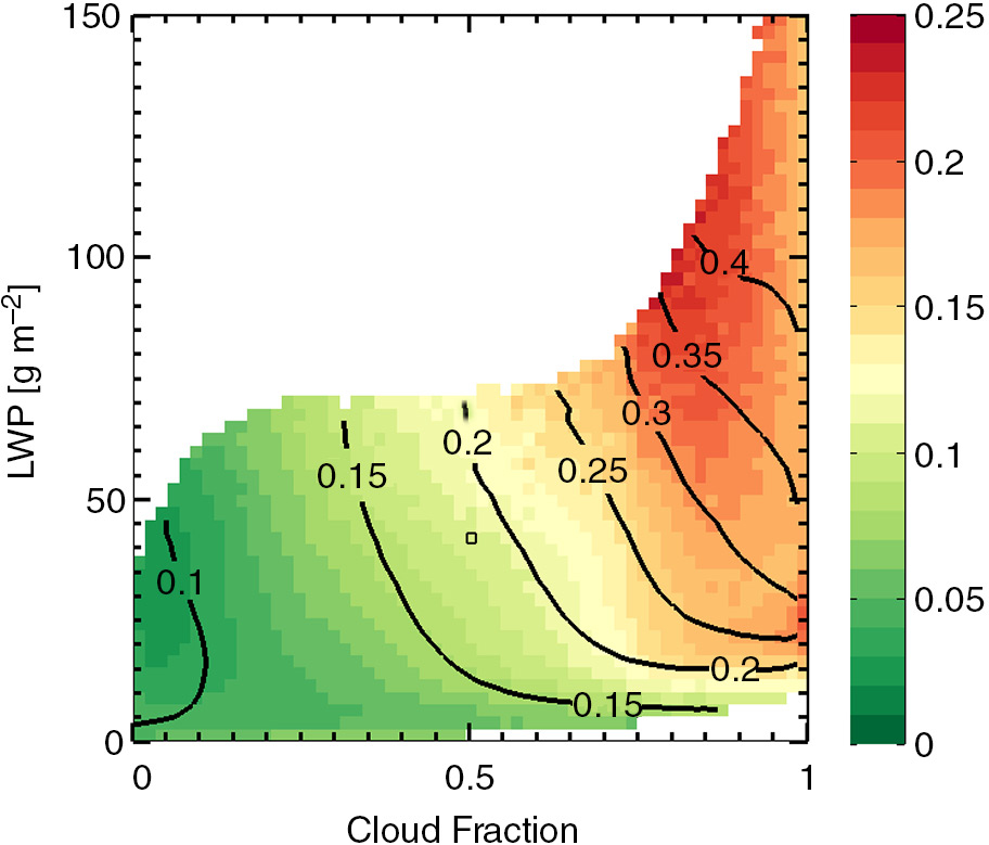
Fig. 1

The standard deviation of albedo increases alongside increasing values of albedo. The highest variability in albedo at a constant f _c and LWP is, however, found at f _c >0.75 and LWP >50 g m⁻² and then decreases slightly closer to f _c =1. At low values of f _c the standard deviation in albedo is small, indicating that clear-sky effects contribute substantially less to the variability in albedo over global ocean compared with differences in cloud albedo. This is in agreement with previous results by Loeb and Kato (2002).

3.2. The high and low albedo footprint

From the complete data set of observations of albedo, it is possible to isolate the aerosol-induced variability in albedo by creating an additional data set of Δα at near-constant values f _c and LWP termed $\mathrm{\Delta }{\alpha }_{f_c,\text{LWP}}$. This is achieved by subtracting the mean albedo from all albedo values in every grid point in Fig. 1, that is, for every small range of f _c and LWP. The resulting albedo perturbations can be represented as a probability density function (PDF) of $\mathrm{\Delta }{\alpha }_{f_c,\text{LWP}}$ at each point in f _c-LWP-space. As an example, Fig. 2 shows the resulting PDF for the grid point at f _c =0.5 and LWP=40 g m⁻².

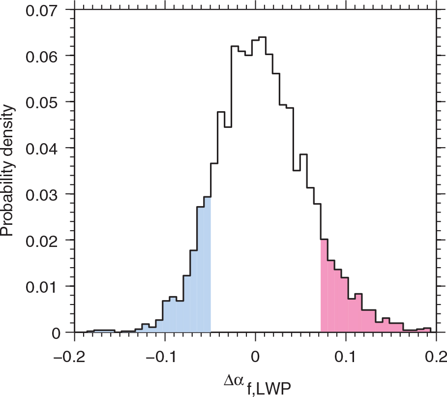
Fig. 2

As indicated by the distribution of values in Fig. 2, we note that the PDF of $\mathrm{\Delta }{\alpha }_{f_c,\text{LWP}}$ at each grid point in f _c-LWP-space contains information about scenes which have negative and positive albedo perturbations for near-constant values of f _c and LWP. While we have not included any information on the atmospheric aerosol loading, by the constraint placed on the analysis in terms of f _c and LWP, this spread is expected to be caused by differences in clear-sky scattering of aerosols and in the optical properties of clouds related to differences in the cloud droplet number concentration.

Every value of $\mathrm{\Delta }{\alpha }_{f_c,\text{LWP}}$ directly or indirectly contains information about differences in the atmospheric aerosol concentration, but the tails of the distribution correspond by definition to cases where the albedo is most perturbed. Therefore, we first focus on the values of $\mathrm{\Delta }{\alpha }_{f_c,\text{LWP}}$ which fall above and below the 90th and 10th percentiles, respectively. Since these extreme values of $\mathrm{\Delta }{\alpha }_{f_c,\text{LWP}}$ can be tied back to their original geographical position, by applying G, we can also study their geographical distribution. As such, we apply G to every value of $\mathrm{\Delta }{\alpha }_{f_c,\text{LWP}}$ that falls above and below the 90th and 10th percentiles, respectively, for each grid point in f _c-LWP-space and move those values back to geographical space. We then express the results as a ratio between the resulting number of $\mathrm{\Delta }{\alpha }_{i,j}$-values and the total number of albedo values available at each 1°×1° degree grid point on the globe to obtain an estimate of the fraction of days which satisfy the initial sampling, and for which a regional albedo perturbation, independent of variations in f _c and LWP, is below or above the 90th and 10th percentiles, respectively.

Figure 3a and b shows the fraction of days for which a region has an albedo perturbation above or below the 90th and 10th percentiles, respectively, independent of variations in f _c and LWP. The results indicate that positive albedo perturbations generally tend to cluster close to coastal areas and near known sources of both natural and anthropogenic aerosols.

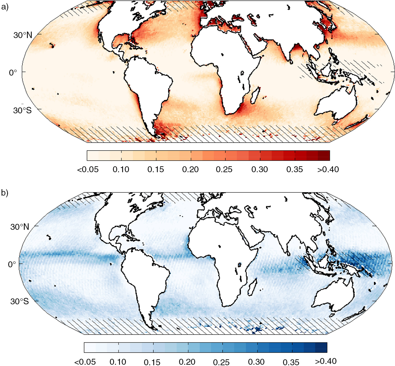
Fig. 3

We note that if the distribution of albedo perturbations exemplified by one pair of f _c and LWP values in Fig. 2 was purely random noise due to instrumental uncertainty, or random retrieval bias, then we would expect the maps in Fig. 3 to be relatively featureless. Instead, several key regions can be identified by their relatively high frequency of strong albedo perturbations. For example, the Chilean smelter region results in a strong increase in albedo downwind and along the west coast of Chile and Peru. A similar example is found along the east coast of Brazil and along both the east and west coast of the United States. A high frequency of strongly positive albedo perturbations is also seen in the Gulf of Mexico, for large parts of the ocean areas surrounding Europe, and in the outflow of polluted air from China. Also clearly visible are the Bay of Bengal, the Indian west-coast, South African and Namibian outflows, and the eastern coast of Australia.

Negative albedo perturbations, shown in Fig. 3b, occur more frequently over remote ocean areas which can be assumed to be cleaner than near-coastal areas. Negative perturbations are also more frequent over equatorial areas. This may indicate that these areas are very clean because of their remote location but may also point to the efficient removal mechanism of aerosols through precipitation. We return to the interpretation of the negative albedo perturbations in Section 4 of the paper.

3.3. Magnitude of global albedo perturbations

In Fig. 3a and b, it is possible to separately encompass areas with very high frequency of high and low albedo perturbations. By selecting all areas in Fig. 3a and b with frequency values larger than 0.3, we construct a new PDF of all albedo perturbations in these regions. The result is shown in Fig. 4. The two resulting distributions show that even if the regions show a high frequency of scenes appearing above the 90th percentile of each PDF of $\mathrm{\Delta }{\alpha }_{f_c,\text{LWP}}$, the PDF of all values in these regions will still display a distribution which may be both negative and positive, that is, indicating a temporal variability related to intermittent sources and sinks of aerosols. Interestingly, the regions corresponding to a high frequency of large and positive albedo perturbations (every 1°×1° grid cell in Fig. 3a with a value higher than 0.3) show a different PDF of the perturbations than the regions corresponding to a high frequency of large and negative perturbations (every 1°×1° grid cell in Fig. 3b with a value higher than 0.3). Although the most frequent albedo perturbation value in these, what we may call polluted, regions is approximately 0.01, the PDF is strongly skewed which indicates that the albedo perturbation can become very large in these areas, and in some cases reach values above 0.1. Assuming a mean solar insolation of 340 W m⁻², this amounts to a substantial difference in the local radiative effect of over −30 W m⁻².

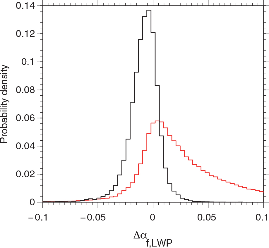
Fig. 4

The PDF of regions that are dominated by a high frequency of negative albedo perturbations is more Gaussian, but slightly skewed towards negative values. We also note that the frequency of negative albedo perturbations converges for both PDFs, that is, there is a lower limit set by the very-clean, clear-sky case over ocean.

Following the above-described procedure, an integrated magnitude of the albedo perturbations globally can also be obtained. We achieve this by again applying G to $\mathrm{\Delta }{\alpha }_{f_c,\text{LWP}}$ for all values in f _c-LWP-space to move them back to their corresponding location in geographical space. This results in a local PDF of Δα at each 1°×1° grid point globally, similar to the two PDFs shown in Fig. 4. As an example, by integrating the two PDFs in Fig. 4, which represent the regions which most frequently above and below the 90th and 10th percentiles, a total albedo perturbation of 0.02 and −0.02, respectively, is obtained. The integral of the local PDF at every 1°×1° grid point globally is shown in Fig. 5. This analysis reveals that the regions outlined as having a high frequency of high albedo perturbations in Section 3.2 show a strong magnitude of these perturbations of 0.02 and above. Assuming a mean solar insolation of 340 W m⁻², this represents a more than −7 W m⁻² local radiative effect. Furthermore, the map of albedo perturbations shows differences down to a level of 0.003 on a regional scale, indicating that when the observational record of albedo is constrained with respect to f _c and LWP, it is possible to detect very small differences in albedo that are comparable to the detection limit of CERES (Wielicki et al., 1996).

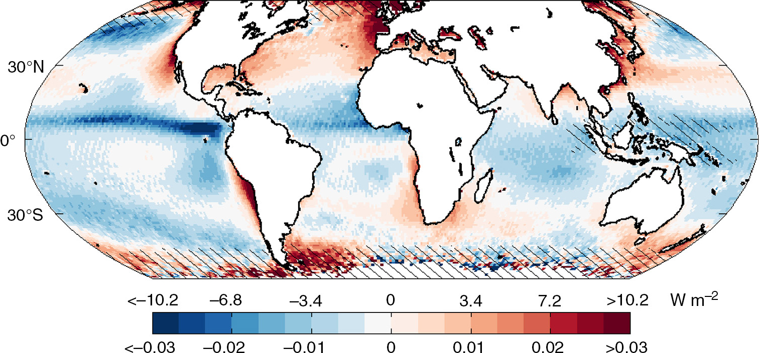
Fig. 5

4. Discussion

By studying the extremes of the probability distribution of albedo perturbations at near-constant values of f _c and LWP, we show that a global and geographically coherent pattern of albedo changes can be identified. Although the limits of 90th and 10th percentiles were empirically chosen, any symmetric pair of percentile limits yields the same results as the one discussed in this study, although the regions of high and low frequency of deviations in Fig. 2 will be larger. The choices of 10th and 90th percentiles represent what we may consider as extreme values of a PDF, and it is interesting to note that the positive component of these extreme values is found close to coastal areas, and near sources of anthropogenic pollution. In such regions, the frequency of occurrence of high albedo perturbation is typically higher than 0.3, that is, of the total amount of days in the study period, 30% can be considered to have an extreme albedo perturbation. We also show that these extremes correspond to a substantial difference in albedo. These albedo perturbations, shown in Fig. 5, are not dependent on any chosen percentile limit, but represent the integrated effect of differences in clear and cloudy sky reflection of sunlight. As such, it can be seen as a total radiative perturbation pattern which is independent of f _c and LWP.

The method of analysis does not separate between direct and indirect effects of aerosols on albedo. However, we note that the areas of positive albedo perturbations agree qualitatively well with previously established areas of liquid clouds with high cloud droplet number concentrations (Bennartz, 2007).

Although the variability caused by differences in the atmospheric aerosol loading cannot be purely isolated because the effect of a varying solar zenith angle cannot be accounted for, the presence of large differences along latitude bands suggest that solar zenith angles are not the dominant factor in determining the strength or the location of the observed perturbations. This is also supported by the fact that the highest latitudes (i.e. regions with the highest solar zenith angles) do not show the highest frequency of high albedo perturbations. We further note that for a plane parallel liquid cloud (Wood, 2012), the difference in solar zenith angle must be more than 30 degrees to introduce an albedo perturbation comparable to the standard deviation of the distribution shown in Fig. 2.

Cloud heterogeneity may still be a factor influencing the frequency of positive albedo perturbations, but since this is reported to be mainly occurring for cumulus clouds in the trade wind regions (Rossow et al., 2002), there is no reason that this should introduce the spatially coherent pattern shown in Fig. 3a. It can therefore be assumed that the observed spatial distributions of frequency of positive albedo perturbations are primarily the effect of an aerosol variability causing a difference in the amount of clear-sky reflected sunlight, and in cloud albedo through an aerosol impact on cloud optical properties.

While an anthropogenic contribution to positive deviations might be suggested because of the location and scale of the geographically coherent positive albedo perturbations, we also note that negative perturbations correspond to regions of intense precipitation from warm liquid clouds with cloud top heights less than 3 km (cf. Fig. 6). Specifically, relative minima in albedo are located in regions with high precipitation rates over the eastern Equatorial Pacific and downwind of the major stratocumulus regions. For example, the North Atlantic generally has lower precipitation rates for warm liquid clouds than other ocean basins, which might explain the relatively higher albedos observed in this region. The causal pathways which explain the albedo perturbations are therefore complicated. One possibility is of course the well-known effect of aerosols impacting the precipitation efficiency of warm clouds (Albrecht, 1989), but high precipitation rates will also impact negatively on the aerosol particle population and have been outlined as an important removal mechanism of potential cloud condensation nuclei (Wood et al., 2012; Berner et al., 2013). The bottom line is that consideration of aerosol sources, or lack thereof, might not fully explain the observed pattern, and that sinks may be equally important.

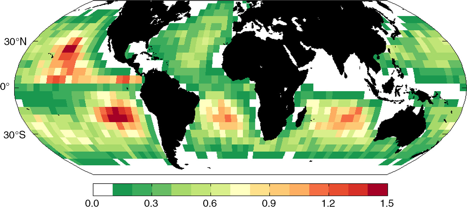
Fig. 6

Strong and negative albedo perturbations are also detected in regions which are not necessarily associated with aerosol sinks, for example, in the Saharan outflow of dust aerosols over the Atlantic, but aerosols in this area are generally considered to cause an increase in the amount of reflected sunlight. However, in the way the analysis is constructed, as a relative metric, this negative signal is not entirely unexpected. Scattering of sunlight by dust aerosols is mainly a clear-sky effect, but the cloud fraction of the ocean areas typically associated with the Saharan dust outflow is relatively high. In our analysis (only warm cloud scenes), the mean cloud fraction ranges typically between 0.5 and 0.7 (not explicitly shown; the higher limit is typically found in the Gulf of Guinea), which means that clear-sky effects constitute less than half of the total albedo over these regions. We also know that albedo variability for cloudy skies greatly dominates over clear-sky variability (see Fig. 1). As such, it is the cloudy-sky portion that will determine the strength of the albedo perturbations shown in these regions. Therefore, as the analysis shows, these regions are not the brightest in the range of cloud fraction and LWP values that dominate these areas, and compared with other similar cloud scenes they typically show a lower albedo.

If the observed pattern of positive albedo deviations is assumed to be mainly caused by the proximity of aerosol sources, this could be related to a total microphysical radiative effect relative to the mean cloud scene at constant f _c and LWP. Assuming a mean solar insolation of 340 W m⁻², all positive albedo perturbations represent a global mean radiative effect of −3.3 W m⁻². However, the question still remains to what extent the perturbations can be attributed to anthropogenic factors. A simple approximation is to assume that albedo scales linearly with the atmospheric aerosol loading and that some fractions of the aerosols are anthropogenic. Sekiguchi et al. (2003) assume a 30% global increase of aerosols due to anthropogenic activity since pre-industrial times. This translates to a present-day anthropogenic aerosol fraction of 23%. Although this number could be used to translate the positive albedo perturbations to an anthropogenic effect, it would also imply that the negative albedo perturbations are anthropogenic in origin, and they appear to be more related to sink processes that influence the albedo. Assuming a relation only to positive perturbations, this would correspond to an anthropogenic radiative effect of −0.8 W m⁻². A more realistic approach would be to assume that the anthropogenic aerosol fraction shows a regional distribution. Recently, Bellouin et al. (2013) described a method by which the anthropogenic fraction of aerosol optical depth was estimated using the European Centre for Medium-Range Weather Forecasts MACC re-analysis. However, even though this kind of analysis could be used in a diagnostic way to understand the possible anthropogenic contribution to the albedo perturbations, we emphasise again that an anthropogenic forcing, as defined by IPCC (2013), would not be obtainable since we are examining the present-day perturbations relative to the mean albedo at small ranges of f _c and LWP rather than comparing to an, in this case, unknown pre-industrial state.

Finally, we note that another choice of normalisation, for instance, the most frequent albedo in each small range of f _c and LWP, or a physically or empirically based estimate of a ‘normal’ albedo, may result in a slightly different map of albedo perturbations which may be used to further untangle the question marks related to aerosol-induced changes to albedo. Also, the use of other available satellite observations of albedo, f _c and LWP may as well introduce variations in the presented result. However, the analysis has been repeated using LWP data from the AMSR-E instrument on-board the Aqua satellite, albeit for a shorter time period but with very similar results (not shown).

5. Conclusions

We have analysed all-sky albedo as obtained from satellite-observed radiometric fluxes from CERES to examine its variability independently of variations in cloud fraction and LWP, that is, the two quantities that account for a substantial fraction of the variance in albedo. Here, we show that by analysing albedo perturbations for small ranges of observed cloud fraction and LWP, with the purpose of isolating microphysical variability from that of larger scale variability, a global set of integrated albedo perturbations can be obtained. These perturbations show spatial scale and pattern corresponding largely to known sources of aerosols in coastal regions and to regions of intense precipitation in which aerosol can be assumed to be scavenged by precipitation. We also show that regions identified as having large and positive albedo perturbations can be considered extreme in the sense that for more than 30% of the time, they display an albedo perturbation which lies above the 90th percentile of global albedo perturbations, independent of variations in cloud fraction and LWP. We show that this can amount to a substantial integrated local radiative effect of −7 W m⁻², and in some instances even higher.

We emphasise that the purpose of the present analysis is to examine the geographical pattern of radiative perturbations that exists in the global data set of observations of albedo. While an anthropogenic contribution to these positive deviations might be suggested because of the location and scale of the geographically coherent patches, it is imperative to carefully quantify or eliminate all other possible causal factors before the anthropogenic contribution can be evaluated. On the other hand, the geographical pattern obtained can be used to diagnostically evaluate the performance of global climate models in terms of representing regional albedo perturbations due to microphysical effects. Furthermore, models could also be used to understand the natural and anthropogenic component of the observed albedo perturbation pattern.

Finally, we note that the small magnitudes of shifts in albedo that are revealed by examining the geographical distribution of albedo perturbations demonstrate a sensitivity of about 0.003 of change in albedo out of an average albedo of 100 times that number. While we do not herein proceed to do a formal analysis of detection limits of this method, it may serve as a complimentary way to enhance the standard signal-to-noise approach of, e.g. Seidel et al. (2014). As such, this method may also be useful, and generally applicable, for the detection and quantification of small spatially distributed perturbations of a dependent variable in noisy global data sets.