
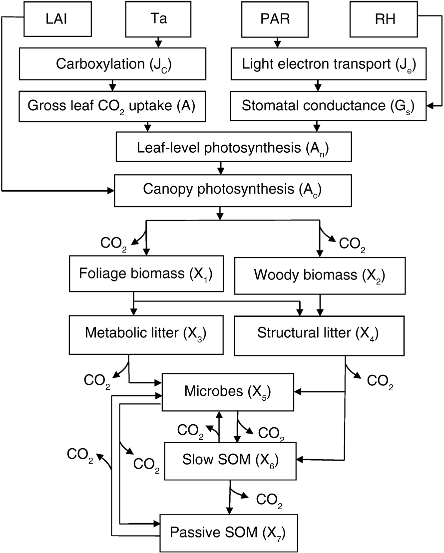
Fig. 1
Schematic diagram of the terrestrial ecosystem (TECO) model with canopy photosynthesis and vegetation–soil C transfer models for data assimilation. LAI, leaf area index; Ta, air temperature; PAR, photosynthetically active radiation; RH, relative humidity. The canopy photosynthesis model is used to describe gross primary production (GPP) calculated by leaf area index (LAI) and the carbon influx of the top leaf layer (A n). The latter was calculated by Leuning model (Leuning, 1995) using gross leaf CO2 uptake (A) and stomatal conductance (G s). For C3 plants, A is calculated by the rates of carboxylation enzymes (J c) and light electron transport rates (J e) according to a model developed by Farquhar et al. (1980).
Table 1. Symbols and description of parameters, their intervals (lower and upper limits) and units in this data assimilation
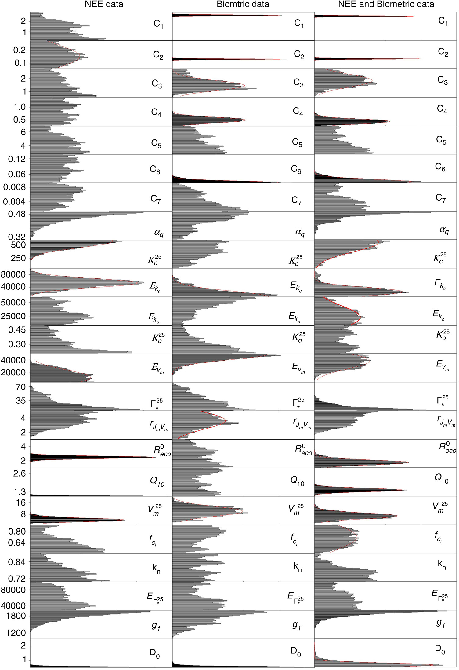
Fig. 2
Posterior distributions of 23 parameters using net ecosystem exchange (NEE) data (Experiment 1), biometric data (Experiment 2) and both NEE and biometric data (Experiment 3) for parameter constrains. The normal distribution curves (red line) represent that the parameters are well constrained by the datasets. See Table 1 for parameter abbreviations and units.
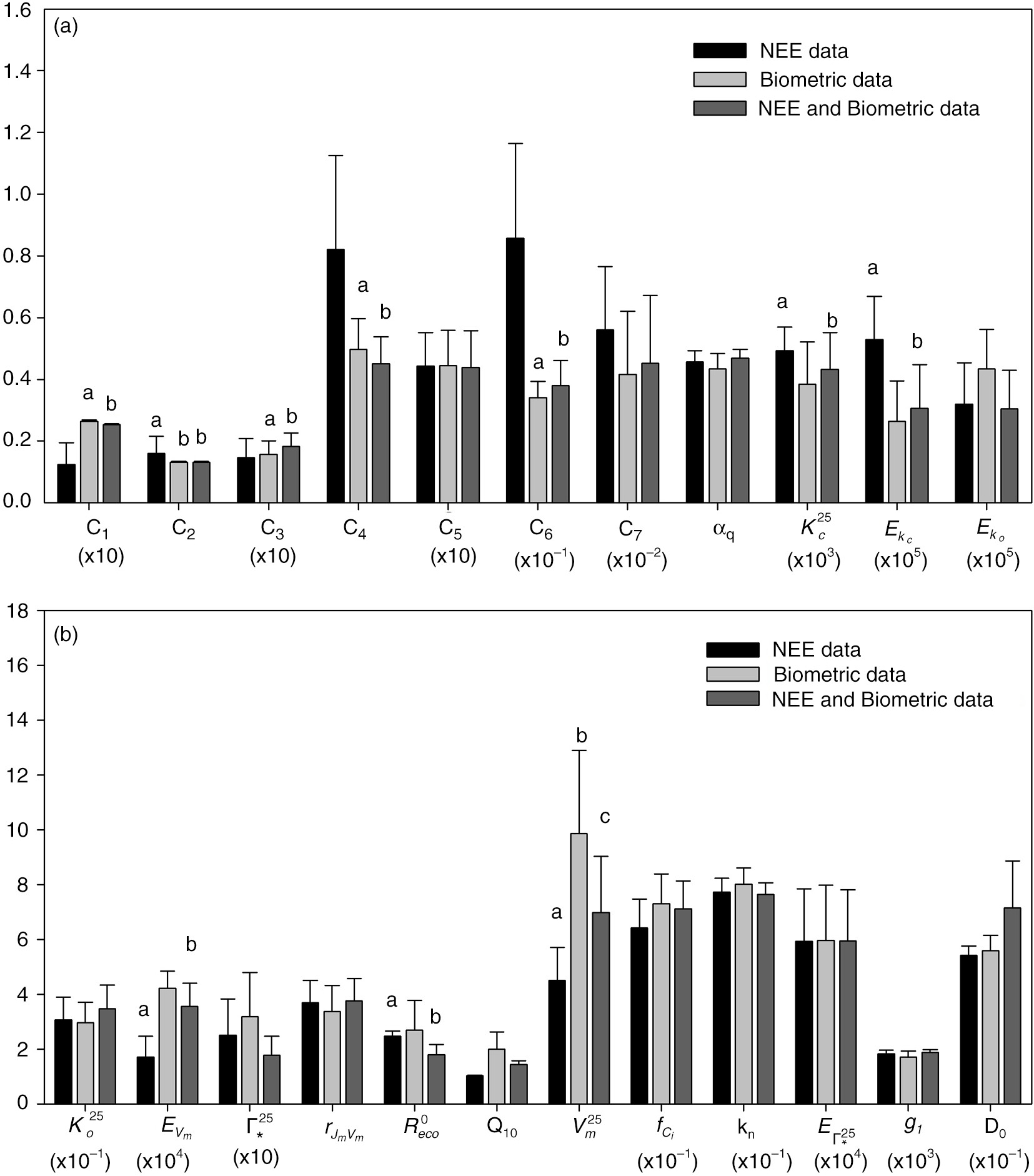
Fig. 3
Maximum likelihood estimators (MLEs) (or means for unconstrained parameters) for 23 parameters in three experiments (11 parameters are shown in panel a and the rest 12 parameters are shown in panel b). Error bars represent standard deviations (SDs) of parameters calculated from 50 000 samples of Metropolis–Hastings (M–H) simulation. The letters a, b and c above the bars indicate statistical significance (α=0.05). See Table 1 for parameter abbreviations and units.
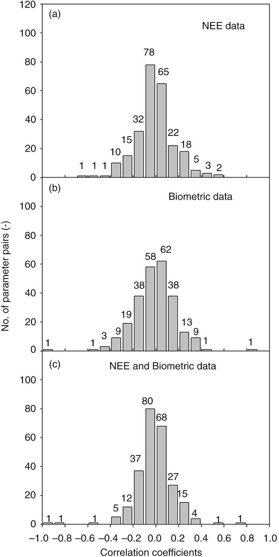
Fig. 4
The frequency distributions of correlation coefficient between every possible parameter pair in three experiments (a) NEE data, (b) biometric data and (c) NEE and biometric data combined.
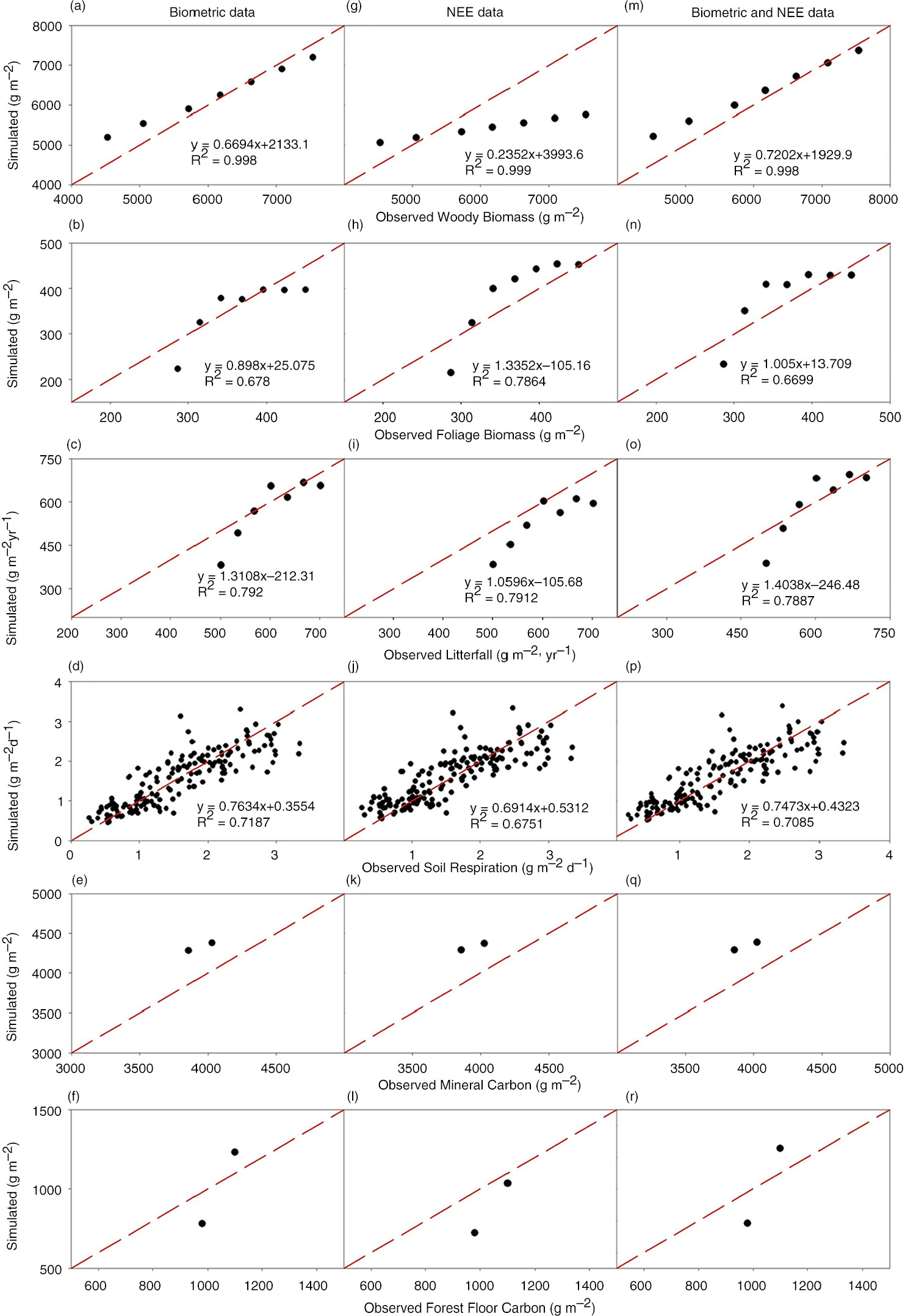
Fig. 5
Comparisons between simulated and observed woody biomass (a, g and m), foliage biomass (b, h and n), litterfall (c, i and o), soil respiration (d, j and p), mineral carbon (e, k and q), and forest floor C (f, l and r) from three experiments (NEE data, biometric data, and NEE and biometric data).
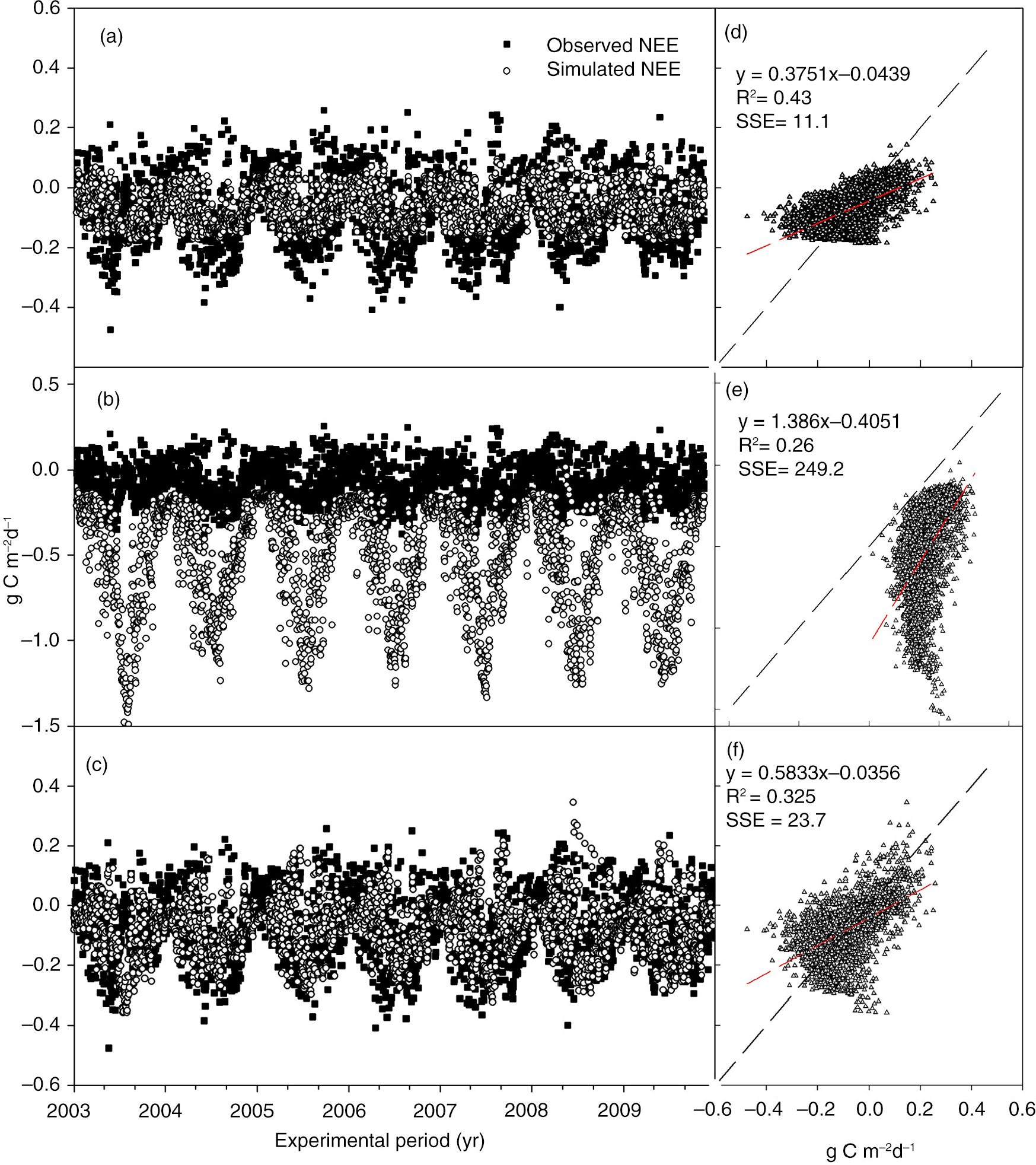
Fig. 6
Comparison of simulated and observed NEE data (from 2003 to 2010) based on three experiments (NEE data, biometric data, and NEE and biometric data combined). The simulated and observed NEE data derived from NEE data, biometric data, combined NEE and biometric data are listed in panels a, b and c; the relationships between simulated and observed NEE data are shown in panels d, e and f, respectively. SSE is sum of squares error.
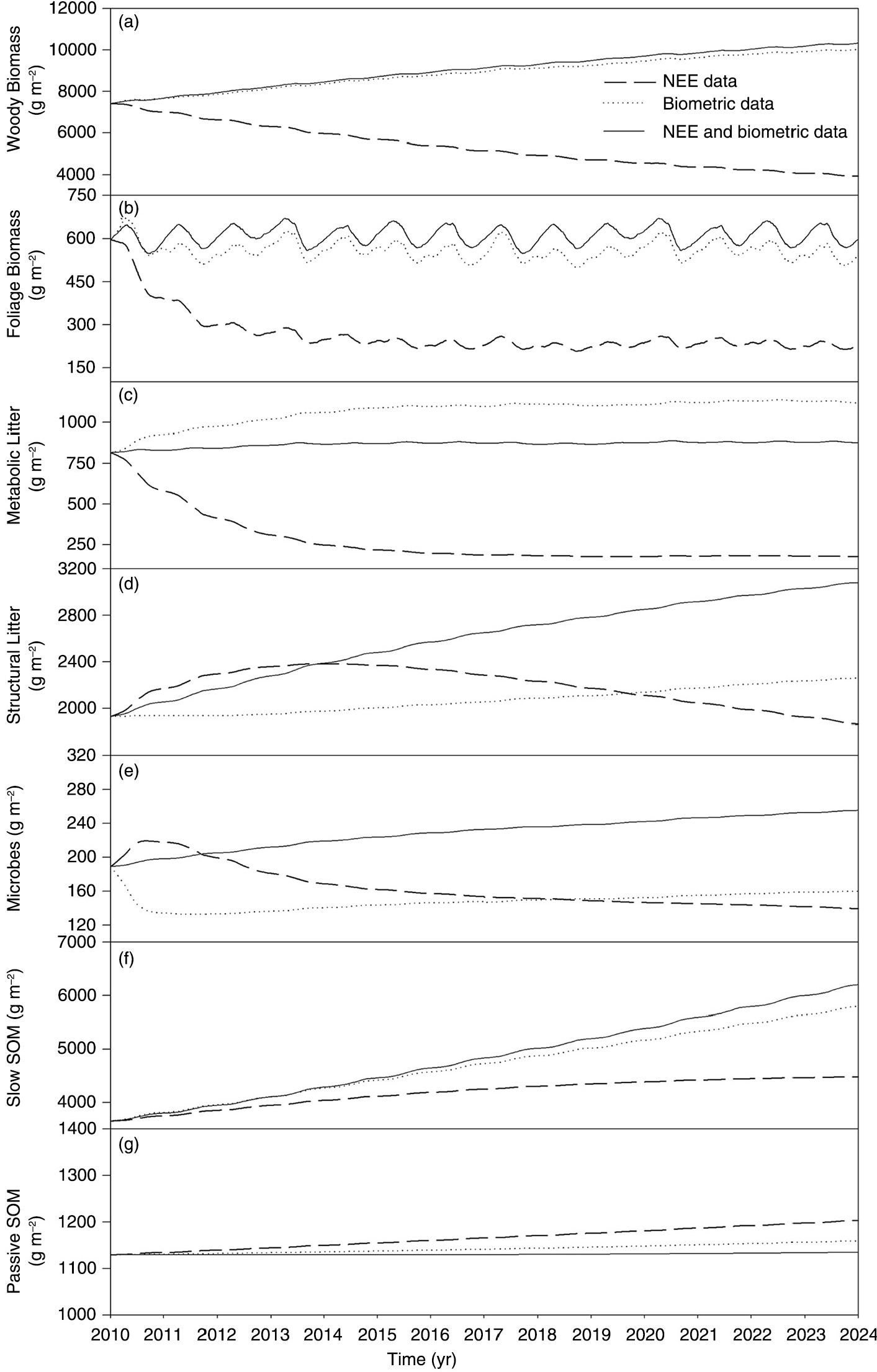
Fig. 7
Predicted woody biomass (a), foliage biomass (b), metabolic litter (c), structural litter (d), microbes (e), slow SOM (f), and passive SOM (g) from 2010 to 2023 using the parameter values of MLEs (well-constrained parameters) and means (poorly constrained parameters) from Experiment 1, 2 and 3.
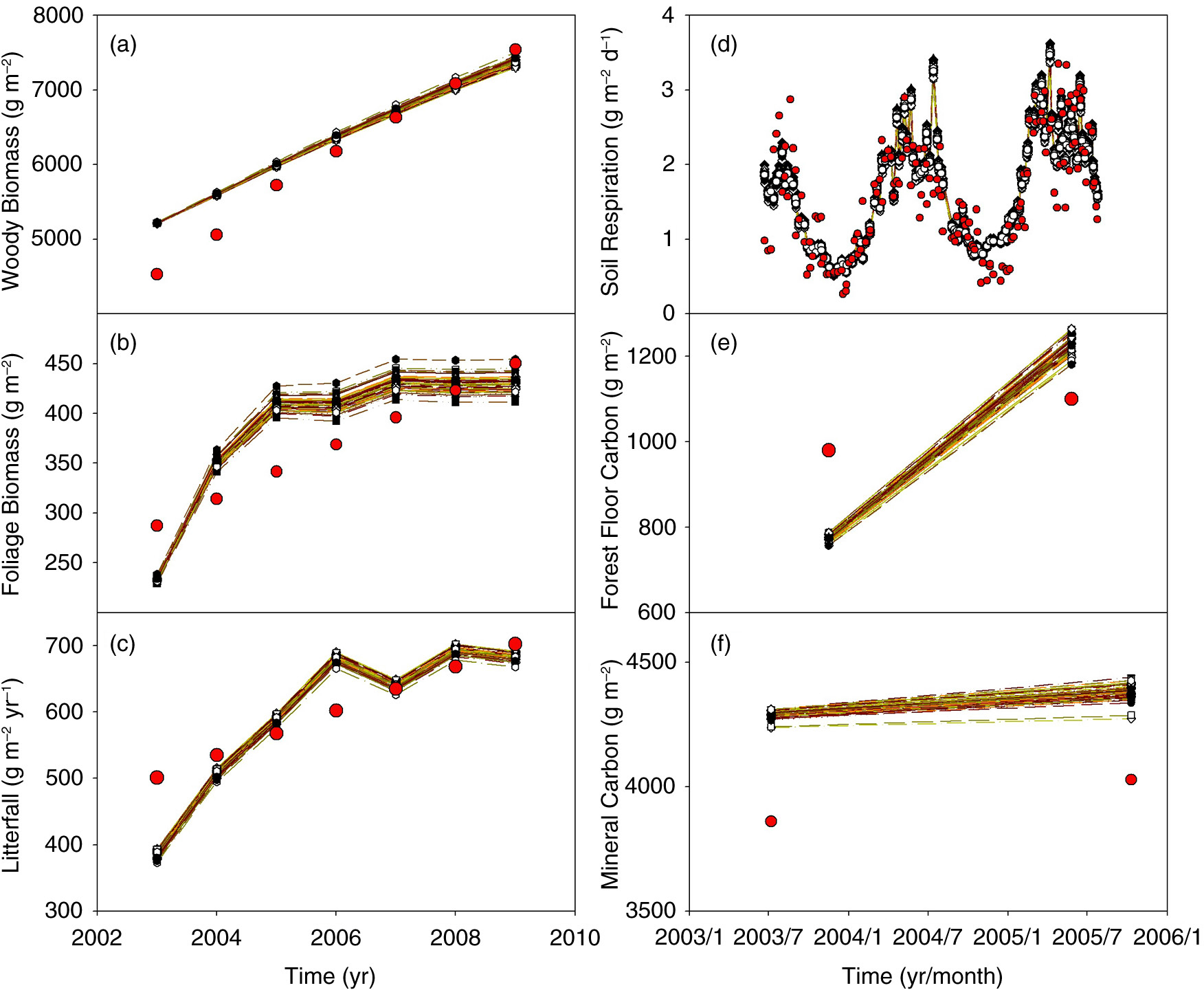
Fig. 8
C pools (i.e. woody biomass, foliage biomass, litterfall, mineral carbon and forest floor carbon) and soil respiration simulated by using 100 random parameters sampled from all 5000 parameters are listed in panels a, b, c, d, e and f. The red solid circles represent observed data and other symbols (line with point, 100 in all) represent simulated data in each panel.