
1. Introduction
As a consequence of human activities, such as fossil fuel combustion and land use changes, the dramatic and unprecedented changes have occurred in the global chemical and physical environment, including well-documented increases in atmospheric carbon dioxide (CO2) concentration and air temperature (IPCC, 2007). These alterations are likely to alter precipitation regimes (e.g. frequency and magnitude) and increase the inter- and intra-annual variability of precipitation due to amplification of the global hydrological cycle (Seneviratne et al., 2006; IPCC, 2007). Rapid climate change poses a major challenge for ecosystem scientists and managers as they attempt to forecast the future states of ecosystems and the climate. One of the main uncertainties in projecting the future climate is to accurately quantify the climate-carbon (C) cycle feedback and the underlying processes (Luo et al., 2009).
Recently, significant progress has been made in improving model structure and optimising methodologies to couple climate change with the C cycle (Wang et al., 2009; Luo et al., 2011). For instance, a ‘model-data fusion’ or data assimilation approach can both highlight model deficiencies and integrate different data streams by parameters it constrains (Wang et al., 2009; Keenan et al., 2013). The Bayesian paradigm allows the researchers to generate posterior probability density functions (PDFs) for model parameters by assimilating prior PDFs and measurements (Dowd and Meyer, 2003). Markov chain Monte Carlo (MCMC) technique is one of the most frequently used optimisation methods in data assimilation studies to evaluate the full joint distribution of target variables with the Metropolis criterion (Xu et al., 2006; Luo et al., 2011), which can be used to determine most probable values, quantiles and other summaries of uncertainty (Luo et al., 2011). Braswell et al. (2005), for example, applied the Bayesian framework to evaluate the information contents contained in net ecosystem exchange (NEE) observations using a simplified photosynthesis and evapotranspiration model (SIPNET). Xu et al. (2006) evaluated uncertainty in parameter estimation and projected C sinks using a terrestrial ecosystem (TECO, vegetation–soil C transfer only) model with six datasets under both ambient CO2 (350 ppm) and elevated CO2 (550 ppm) plots at the Duke Forest Free-Air CO2 Experiment (FACE). Although the main biological processes have long been identified in terrestrial C cycling, it is still insufficient to use integrated processes (e.g. photosynthesis, respiration, C sequestration) with different data streams to improve parameter estimation and forecast the future states of ecosystems and the climate.
Flux- and biometric-based data are two major data sources for studying terrestrial C cycling, in which some efforts have been made in data assimilation. For example, daily NEE data at seasonal time scales could greatly constrain most model parameters of photosynthesis and respiration processes (Braswell et al., 2005). Biometric data are effective in constraining C transfer coefficients from plants pools in leaves, roots and wood, but were poor from metabolic litter, microbial and passive soil organic matter (SOM) (Xu et al., 2006). Long-term forest stem surveys and tree ring data may offer a rich resource on the constraints of slow C processes (Williams et al., 2005). Previous analyses have mainly focused on uncertainties from the lack of data or timescale mismatching between the available data and the estimated parameters (Mo and Beven, 2004), and characterising the error structures in each data stream (Raupach et al., 2005). However, how flux- and biometric-based data affect uncertainties in parameter estimation is largely unclear.
Few studies have currently been conducted to examine the effects of data sources on model parameters and ecosystem C processes. For example, Richardson et al. (2010) have examined the effects of different data streams on parameters and initial C stocks using a Data Assimilation Linked Ecosystem Carbon (DALEC) model. Most parameters and initial model states were poorly constrained by tower-measured fluxes alone. When biometric data (e.g. soil respiration, leaf area index (LAI), woody biomass and litterfall) were added, they largely reduced bias compared with observations and uncertainties on model predictions. Zhang et al. (2010) also evaluated the effects of NEE and biometric data on the constraints of model parameters using TECO model and found that these datasets provided different effectiveness in constraining C transfer coefficients (i.e. plant pools by biometric data and soil pools by NEE) in three forest ecosystems in China. However, previous studies have not considered the uncertainties of the input data thoroughly enough. For example, gross primary production (GPP) was either taken from the outputs of another model in Richardson et al. (2010) or from the self-loop calculation of flux-measured NEE (i.e. GPP=NEE+RE as a photosynthetic input and also taking NEE as the observed data to constrain parameters, where RE is the ecosystem respiration) in Zhang et al. (2010). It is necessary to examine the information contents contained in flux data, biometric data or both when we combine canopy photosynthesis processes with a plant and soil C transfer model to constrain model parameters and initial states as well as model predictions.
This study was designed to examine the information content of flux- and biometric-based data on parameter constraints. We applied a Bayesian probabilistic inversion approach to an evolved TECO combined with a canopy photosynthesis submodel. An MCMC sampling method was used to construct posterior PDFs for all the model parameters. The data include biometric-based data from field experiments (i.e. foliage biomass, woody biomass, litterfall, soil respiration, and C content in litter layers and mineral soil), flux-based data taken from the eddy covariance method [i.e. NEE, air temperature at the top canopy, photosynthetically active radiation (PAR), relative humidity (RH)] and remote sensing data (i.e. LAI). All the data were collected from 2003 to 2009 at a subtropical coniferous plantation in Qianyanzhou, Jiangxi Province, China. Three experiments with different data streams were conducted to parameterise parameters by using NEE data, biometric data and both NEE and biometric data.
2. Materials and methods
2.1. Site information
The Qianyanzhou site (26°44′29′′N, 115°03′29′′E, 100 m above sea level), which belongs to the ChinaFLUX network, is located in Jiangxi Province, China. This site is characterised by a subtropical monsoon climate, while other areas at a similar latitude are arid steppes and deserts (Huang et al., 2007). Based on the meteorological records from 1985 to 2007, the mean annual temperature and precipitation were 17.9°C and 1475 mm, respectively (Wen et al., 2010). The soil parent material consists of red sandstone and mud stone, and the soils are mainly red earth. The original vegetation in the study area was mainly evergreen broadleaf forest, which was destroyed thoroughly at the beginning of the 1980s due to intense deforestation. The current vegetation is a coniferous forest plantation, which is 25 yr old and ~13 m tall. The dominant species are Pinus massoniana, Pinus elliottii and Cunninghamia lanceolata. According to field measurements in August of 2003, the LAI of the plantation was 4.5 (Li et al., 2006a), and the average diameter at breast height (DBH) was 15.4 cm (Li et al., 2006b). The eddy flux observation tower was set up in the plantation in 2001. Around the tower, the forest coverage was 90% within 1 km2 and 70% within 100 km2 (Huang et al., 2007).
2.2. Data sources
The datasets used in this study included climatic and biotic variables (i.e. air temperature at top canopy [T a ], photosynthetically active radiation [PAR], relative humidity [RH] and leaf area index [LAI]); biometric measurements (foliage biomass, woody biomass, litterfall, soil respiration, C content in the litter layers, and mineral soil); and eddy flux data [net CO2 exchange (NEE)] collected from 2003 to 2009 at the Qianyanzhou site (QYZ). In the model, NEE and biometric data sets were served as inversing data, and the other datasets were used as driving data.
NEE data and the corresponding climatic variables were aggregated to an hourly time step from half-hourly data on CO2 flux, T a , PAR and RH, which were downloaded from the Chinese Ecosystem Research Network (CERN, www.cern.ac.cn). The CO2 flux was measured by the eddy covariance technique (Baldocchi et al., 1988). The raw data were preprocessed by rejecting outlier data (∣the value of CO2 flux∣>3 mg CO2 m2 s−1) and nighttime filtering based on the methods of Papale et al. (2006). A Q10 function and a Michaelis–Menten function were then used to model the nighttime respiration and daytime photosynthesis, respectively (Richardson and Hollinger, 2005). Gaps in the CO2 flux data were filled by using these two functions. Further details of the steps were described by Shao et al. (2014).
Yearly woody and foliage biomass were estimated by an allometric equation with DBH. As previous studies reported (Shen, 2006; Li et al., 2006b), both DBHs and biomass (including woody and foliage) of the dominant species were measured in August 2003 and July 2007 at main plots of the QYZ, which were used to establish an allometric equation with biomass and DBHs. For the remaining 5 yr (2004–2006, 2008–2009), we only measured the DBHs of the dominant species and then applied this regression to extrapolate the woody and foliage biomass. According to the allometric relationships between DBHs and biomass from Li et al. (2006b), approximately 93% of the total biomass is woody biomass and the rest is foliage biomass, which includes fine roots and leaves (Ma et al., 2007). Fine roots and leaves were lumped together to reduce the number of parameter values because they have similar residence times (Luo et al., 2003).
Aboveground litter was collected from 100×100 cm baskets with 10 replicates at the QYZ once per month during the growing season (May–October) from 2003 to 2005 (Li et al., 2006b). The collected litter was dried at 70°C for 24 hours and weighed. In this model, we aggregated monthly data to calculate the annual litterfall for inverse analysis, in order to avoid the effect of the extreme wind events on litterfall biomass measurement within individual months. We also used a linear regression method to calculate the aboveground litter biomass of the remaining 5 yr.
Measurement of C content in the forest floor was undertaken using the method described by Schlesinger and Lichter (2001). Soil samples were collected twice from 2×2 m samples with 12 replicates at the QYZ site in December 2003 and August 2005 (Shen, 2006). In each sample, undecomposed plant materials on the soil surface were separated for measurement of C content in the surface litter layers. For soil mineral C, soil samples from four soil layers (0–10, 10–30, 30–60, 60–100 cm) were collected twice in December 2003 and August 2005. The SOC of these samples were measured by the potassium dichromate oxidation titrimetric method.
Soil respiration was measured weekly using a static chamber-gas chromatograph technique from January 2003 to October 2005 (Zhang et al., 2006). Each sampling chamber is composed of a base box (50 cm×50 cm×10 cm) and the chamber box (50 cm×50 cm×50 cm). The base part with U-shape grooves (2 cm wide and 3 cm deep, sealed with adhesive rubber tapes during sampling) was inserted into soil about 24 hours before sampling. Gas samples were taken between 9:00 am and 11:00 am with a 90-mL plastic syringe at 0, 10, 20 and 30 minutes. All samples were taken back to the lab and analysed using a gas chromatographer (HP4890D, Agilent, USA) within the same sampling day. CO2 was separated using a 2 mm 60–80 Porapak column at 200°C, and measured with flame ionisation detector (FID) at 375.55°C, carried with pure nitrogen gas at a flow speed of 30 mL min−1. Flux was calculated from the linear increase of each CO2 sample concentration (r 2≥0.95 for n=4, otherwise the sample was rejected).
LAI data were obtained from the remote sensing data archive in the US Geological Survey (USGS) database (http://www.usgs.gov/). The LAI data were rejected when cloud cover levels were>5%. Consequently, we obtained 194 daily LAI values. In order to reduce the uncertainty, these data were calibrated with measured LAI data collected from 2003 to 2006 at the QYZ site by Song (2007).
2.3. Model description
The TECO model with seven C pools (Luo and Reynolds, 1999) was used in this study. By adding short-term processes of canopy-level photosynthesis (Ac) and ecosystem respiration (Reco) [also called the flux-based ecosystem model (FBEM)], we evolved the model as pathways of C flux with environmental variables in the terrestrial ecosystem (Fig. 1). Canopy photosynthesis was estimated from LAI and leaf-level photosynthesis (Sellers et al., 1992). The latter was described using the model developed by Farquhar et al. (1980) for both carboxylation and electron transport processes together with a stomatal conductance model (Leuning, 1995; Van Wijk et al., 2000; Chang, 2012). See Wu et al. (2009) for more details. Ecosystem respiration was modelled via the widely used Q10 function (Hoff, 1899). Carbon enters the ecosystem via canopy photosynthesis and is portioned into woody and non-woody biomass. Dead plant materials go to metabolic and structural litter compartments, and are decomposed by microbes. Part of the litter C is respired and the rest is converted into slow and passive SOM pools. Carbon transfer coefficients are rate variables that determine the amount of C per unit of mass leaving each of the pools per day, and the inverses of the transfer coefficients are represented as the mean C residence times, which are the key parameters determining the C sequestration capacity of the ecosystem when combined with primary production (Barrett, 2002; Luo et al., 2003; Xu et al., 2006). The C dynamics can be expressed mathematically by the following first-order ordinary differential equation:
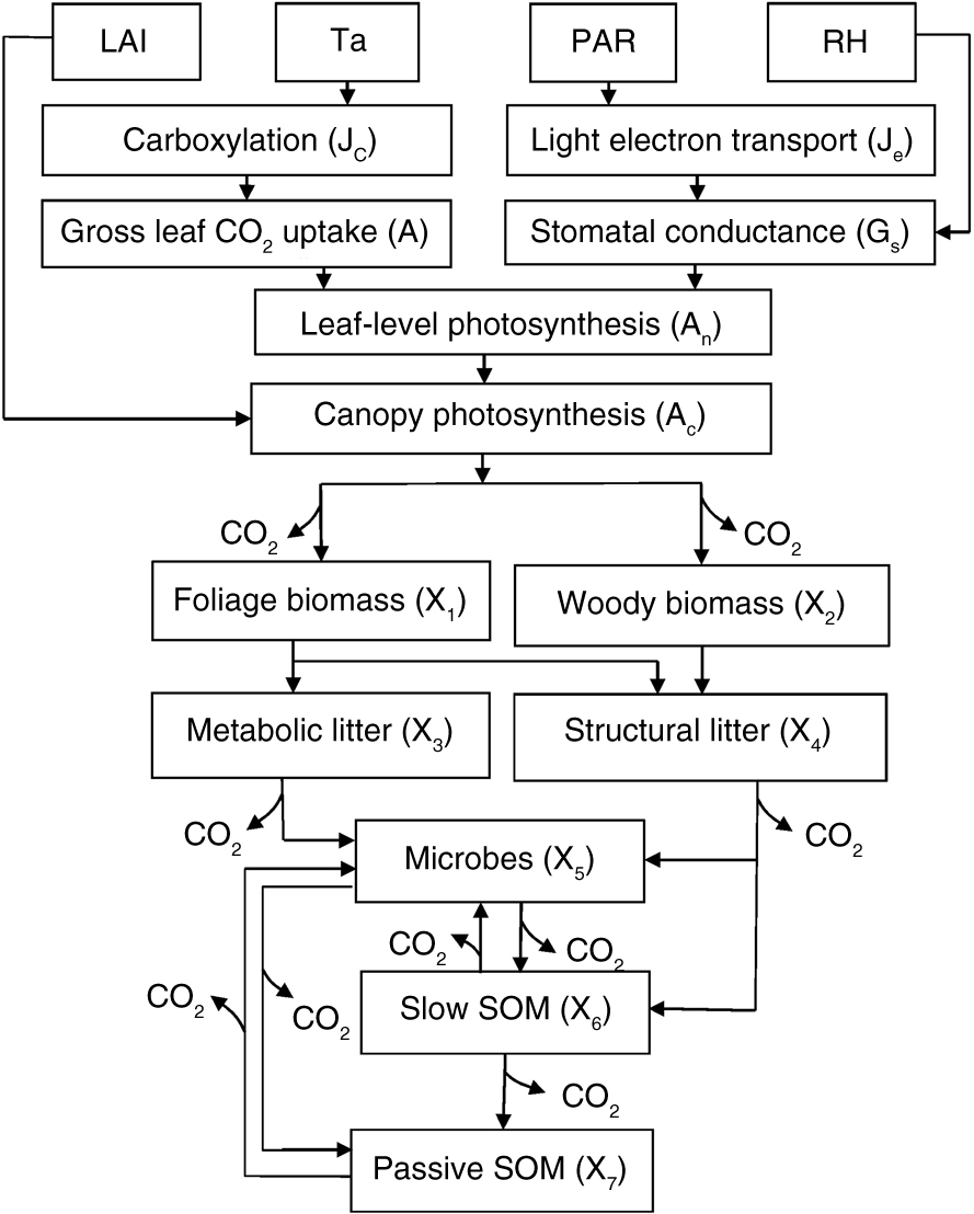
Fig. 1
Schematic diagram of the terrestrial ecosystem (TECO) model with canopy photosynthesis and vegetation–soil C transfer models for data assimilation. LAI, leaf area index; Ta, air temperature; PAR, photosynthetically active radiation; RH, relative humidity. The canopy photosynthesis model is used to describe gross primary production (GPP) calculated by leaf area index (LAI) and the carbon influx of the top leaf layer (A n). The latter was calculated by Leuning model (Leuning, 1995) using gross leaf CO2 uptake (A) and stomatal conductance (G s). For C3 plants, A is calculated by the rates of carboxylation enzymes (J c) and light electron transport rates (J e) according to a model developed by Farquhar et al. (1980).
where X(t)=(X 1 (t), X 2 (t), …, X 7 (t)) T is a 7 × 1 vector, representing C pool sizes in foliage biomass, woody biomass, metabolic litter, structural litter, and microbial, slow and passive SOM at time t, respectively. A and C are 7×7 matrices given by
where diag (C) denotes a 7×7 diagonal matrix with the diagonal entries given by vector c=(c 1, c 2, . . ., c 7) T the components c j (j=1, 2, . . ., 7) represent C transfer coefficients associated with pools X j (j=1, 2, . . . ,7). ζ (t) is a scaling function accounting for temperature and moisture effects on C decomposition. U(t) is C input fixed by canopy-level photosynthesis (Ac, i.e. GPP). B=(0.25, 0.30, 0, 0, 0, 0, 0)T is a vector that determines the allocation of photosynthetically fixed C to non-woody and woody biomass, and the remaining 45% of canopy input C was consumed by plant respiration. X 0=[148 4980 104630 147 3030 1136] T (The unit is g C m−2) represents an initial condition, estimated by the method used in Luo et al. (2001) that is based on an initial steady-state C balance in the TECO model and experimental data at the start of this study. Besides C transfer coefficients, all parameters for calculating Ac and Reco were estimated simultaneously. There were 23 parameters in total to be estimated (Table 1).
Table 1. Symbols and description of parameters, their intervals (lower and upper limits) and units in this data assimilation
2.4. Parameter estimation
We use a Bayesian probabilistic inversion approach to estimate all parameters. The Bayes’ theorem states that the posterior probability density function (PDF) p(c∣Z) of model parameters c can be obtained from prior knowledge of parameters and information generated by a comparison of simulated and observed variables. The theorem can be expressed by
where p(c) is the prior probability density distribution, p( Z) represents the probability of observed data, and p(Z∣c) is the likelihood function for parameter c, which expresses the fit between modelled and observed data.
To apply Bayes’ theorem, we first specified ranges for model parameters as prior knowledge (see Table 1), and the prior PDF p(c) of the parameters was specified as a uniform distribution over the ranges. Lower and upper limits of parameters were set by synthesising of values from the literature, knowledge of the system, the raw model output, and prior information from Luo et al. (2003), Wu et al. (2009) and Zhang et al. (2010). The likelihood function P(Z∣c) was specified according to the distributions of observation errors. Based on the assumption that errors followed a Gaussian distribution with a zero mean, the likelihood function can be expressed as:
where σ2 i is the measurement error variance of each dataset, and, e i (t) is the error for each modelled value Y i (t) compared with the observed value Z i (t) at time t, expressed as:
To calculate Y i (t) from the modelled data X i (t), we use the mapping operator to match the modelled C pool sizes to measurements at time t (Luo et al., 2003; White et al., 2006; Xu et al., 2006; Zhang et al., 2010), and Φ is a 6×7 matrix given as:
For each C pool, the modelled value was expressed as:
whereas simulated NEE was calculated as:
A positive NEE value represents a release of CO2 from the ecosystem, while a negative value denotes a net uptake of CO2 from the atmosphere.
The posterior PDF p(c∣Z) for the model parameters were generated from prior PDFs p(c) with observations Z using an MCMC sampling technique and the Metropolis–Hastings (M–H) algorithm (Metropolis et al., 1953; Hastings, 1970; Gelfand and Smith, 1990) was used as the MCMC sampler. We assumed a Gaussian distribution for the prior probability function p(c) in the parameter space. New proposal parameter points were generated by , whether the new point c new was accepted or not according to the value of the ratio compared with a uniform random number N from 0 to 1. Only if R≥N, the new point was accepted (i.e. c k =c new ); otherwise c k =c k−1 (Xu et al., 2006).
We formally made five parallel runs using the M–H algorithm with 300 000 simulations for each run. Each run started from a random initial point in parameter spaces to eliminate the effect of the initial condition on stochastic sampling. The acceptance rates for the five runs tested by the Gelman–Rubin (G–R) diagnostic method in the three inversion controls ranged from 5 to 10% (Xu et al., 2006). The initial samples (about 3000 for each run) were discarded after the running means and standard deviations (SDs) were stabilised (regarded as the burn-in period). Thus, all accepted samples from five runs after the burn-in periods (about 50 000 samples in total) were used for statistical analysis.
Maximum likelihood estimators (MLEs) are parameter values corresponding to the peaks of their marginal distribution. We calculated the MLEs for the constrained parameters and sample means for unconstrained parameters which we could not calculate MLEs. The SDs of all parameters were also estimated from the posterior PDFs of 50 000 samples to quantify parameter uncertainty. Histograms were constructed from the samples to display the distribution of parameters in the parameter spaces.
2.5. Simulation experiments and uncertainty analysis
Three simulation experiments were designed to constrain all 23 parameters in this study. The first experiment used NEE data only in probabilistic inversion (Experiment 1). The second experiment used biometric data only, which included foliage biomass, woody biomass, litterfall, soil respiration, forest floor C and soil mineral C (Experiment 2). The third experiment used both NEE and biometric data in the inverse analysis (Experiment 3). In order to constrain model parameters by combining the information from datasets with different numbers of points [i.e. mineral C and forest C (two points); wood, foliage and litterfall (seven points); soil respiration (157 points); NEE (122 736 points)] in Experiment 3, we introduced a weighting function: W i =1−N i /N A , where N i (i=1, 2…7) and N A are the numbers of points in dataset i and all data sets, respectively. The cost function was then set as , where P i (Z∣c) is the likelihood function expressed as eq. (4). In our forward simulation, we forecasted the C pool sizes in woody biomass, foliage biomass, metabolic litter, structural litter, microbes, slow SOM and passive SOM from 2010 to 2023. The corresponding optimised parameter values (i.e. MLEs or means) and the C sizes from the last run in the analysis process were served as initial conditions and the weather conditions from 2003 to 2009 were used as input. We randomly selected 100 samples from 50 000 samples with all parameter values in Experiment 3 being used to quantify the uncertainty of C pool sizes.
3. Results
3.1. Parameter estimation
One of the main goals of data assimilation is to identify model parameters by combining models with data. Overall, 6 (Experiment 1), 7 (Experiment 2) and 14 parameters (Experiment 3) were well constrained but with considerable differences in each experiment (Fig. 2). Among the parameters on C transfer coefficients, C 1 , C 2 , C 3 , C 4 and C 6 were well constrained by biometric data and combined NEE and biometric data with steep peaks of frequencies, while only parameter C 2 was constrained by NEE data alone (Fig. 2). In contrast, in the 16 parameters on GPP and ecosystem respiration, E Kc , R 0 eco and V 25 m were well constrained with steep peaks by NEE data and combined NEE and biometric data, but only V 25 m was well constrained by biometric data alone (Fig. 2). Some parameters (e.g. K 25 c and E Vm in Experiment 1, in Experiment 2, K 25 c , E Ko , E Vm and f Ci in Experiment 3) were constrained to some degree but with considerably spread posterior PDFs. Several parameters (e.g. Q 10 , D o ) were constrained well in Experiment 3 but not in others, probably due to the different effectiveness of the data sources in constraining parameters.
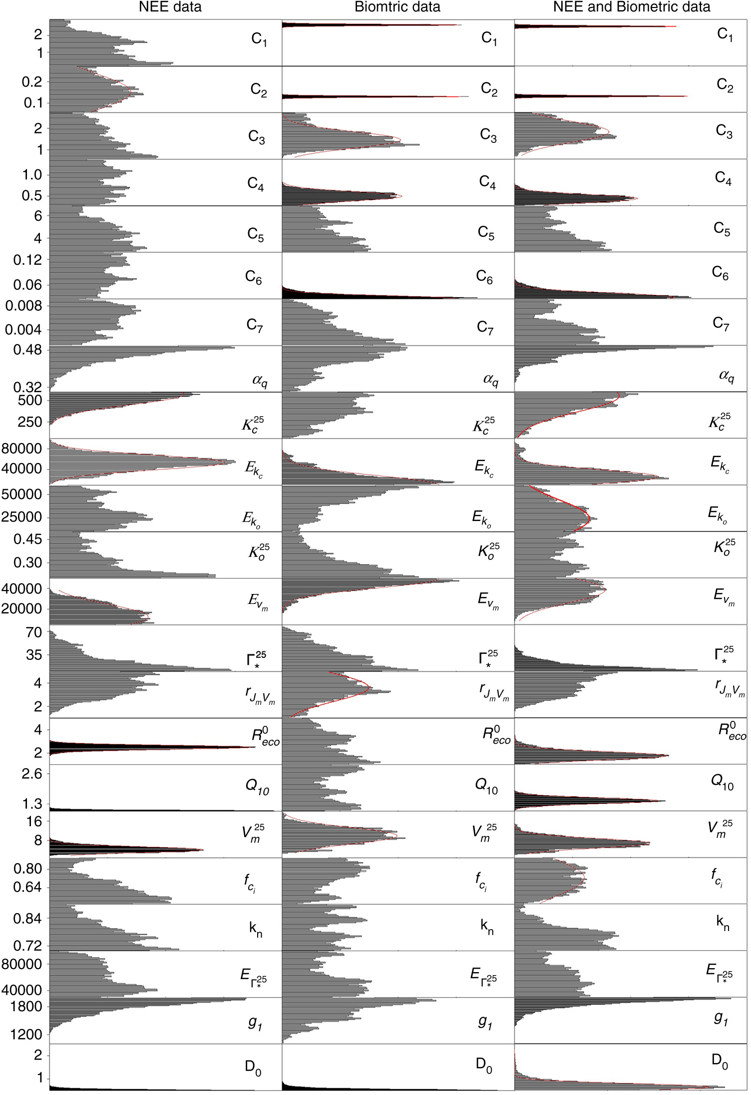
Fig. 2
Posterior distributions of 23 parameters using net ecosystem exchange (NEE) data (Experiment 1), biometric data (Experiment 2) and both NEE and biometric data (Experiment 3) for parameter constrains. The normal distribution curves (red line) represent that the parameters are well constrained by the datasets. See Table 1 for parameter abbreviations and units.
Among the parameters, the poorly constrained parameters C 7 and had the largest variability relative to their range (Fig. 3). The correlation analysis showed that more than 90% of correlations between parameters (∣corr∣) were below 0.3 (Fig. 4). Parameter pairs for high ∣corr∣ values (>0.4) in different experiments were different except for the pair C 3 –C 4 in Experiment 2 (∣corr∣=0.90) and Experiment 3 (∣corr∣=0.89).
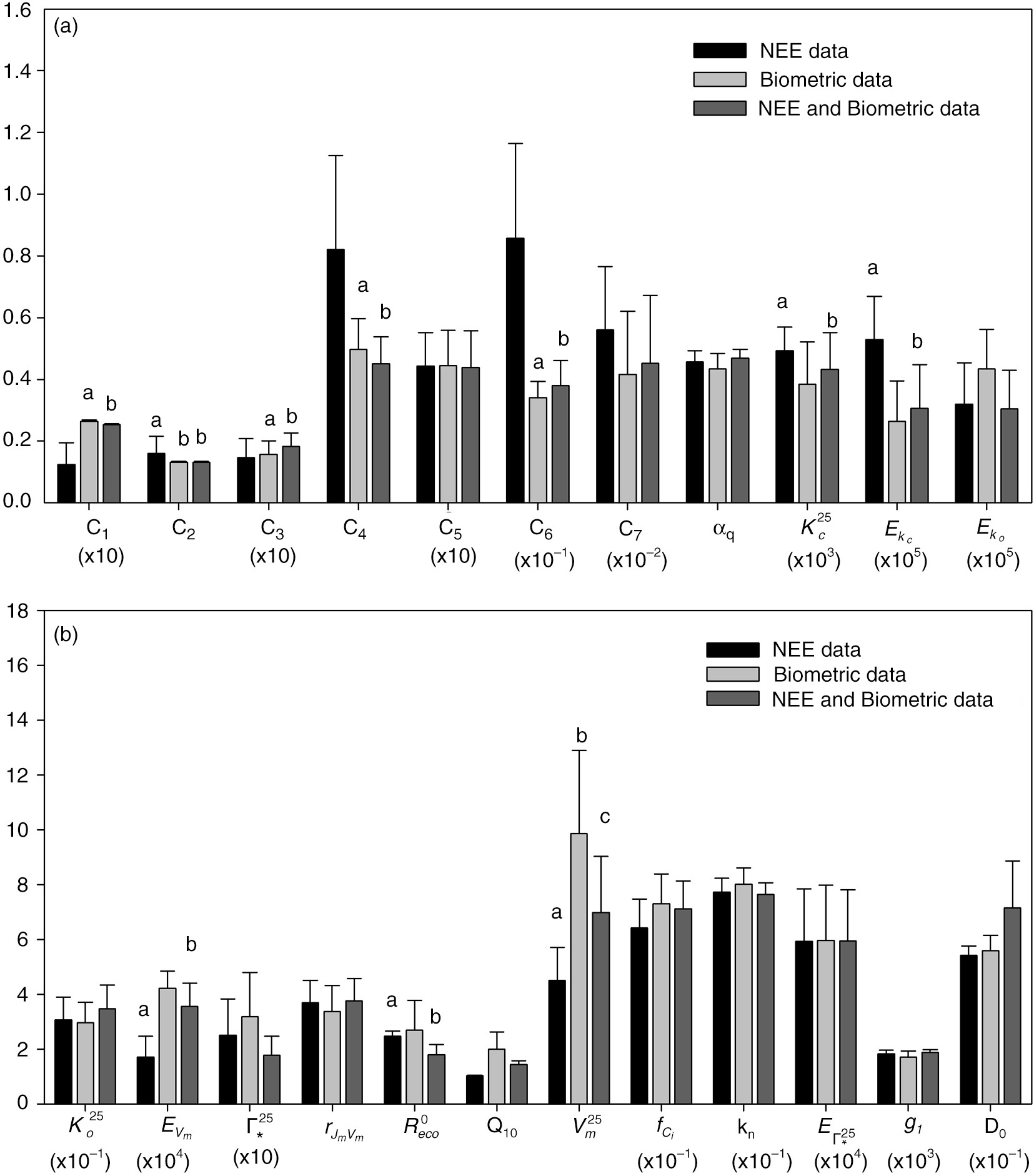
Fig. 3
Maximum likelihood estimators (MLEs) (or means for unconstrained parameters) for 23 parameters in three experiments (11 parameters are shown in panel a and the rest 12 parameters are shown in panel b). Error bars represent standard deviations (SDs) of parameters calculated from 50 000 samples of Metropolis–Hastings (M–H) simulation. The letters a, b and c above the bars indicate statistical significance (α=0.05). See Table 1 for parameter abbreviations and units.
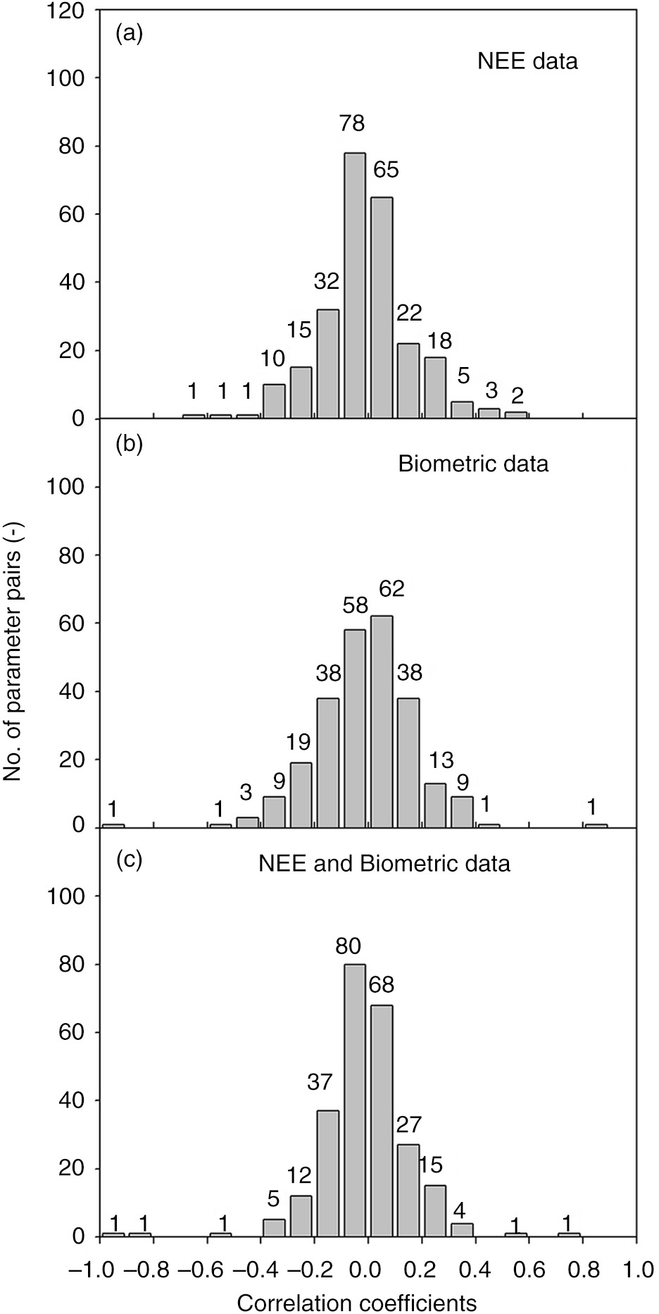
Fig. 4
The frequency distributions of correlation coefficient between every possible parameter pair in three experiments (a) NEE data, (b) biometric data and (c) NEE and biometric data combined.
3.2. Model-data comparison
We evaluated the validity of inverse analysis by comparing model values and the observed data of biometric and NEE data (Figs. 5 and 6). Overall, most C fluxes and pools simulated in the TECO model were closely related to the corresponding observed datasets. However, the simulated and observed biometric data fitted better in Experiment 2 and Experiment 3 than in Experiment 1, while the NEE data fitted more closely in Experiment 1 (Figs. 5 and 6). Large deviations also existed between the simulated and observed foliage biomass (Fig. 5b, h and n), mineral C (Fig. 5e, k and q) and forest floor C (Fig. 5f, i and r), probably due to both a lack of valid data and observation errors.
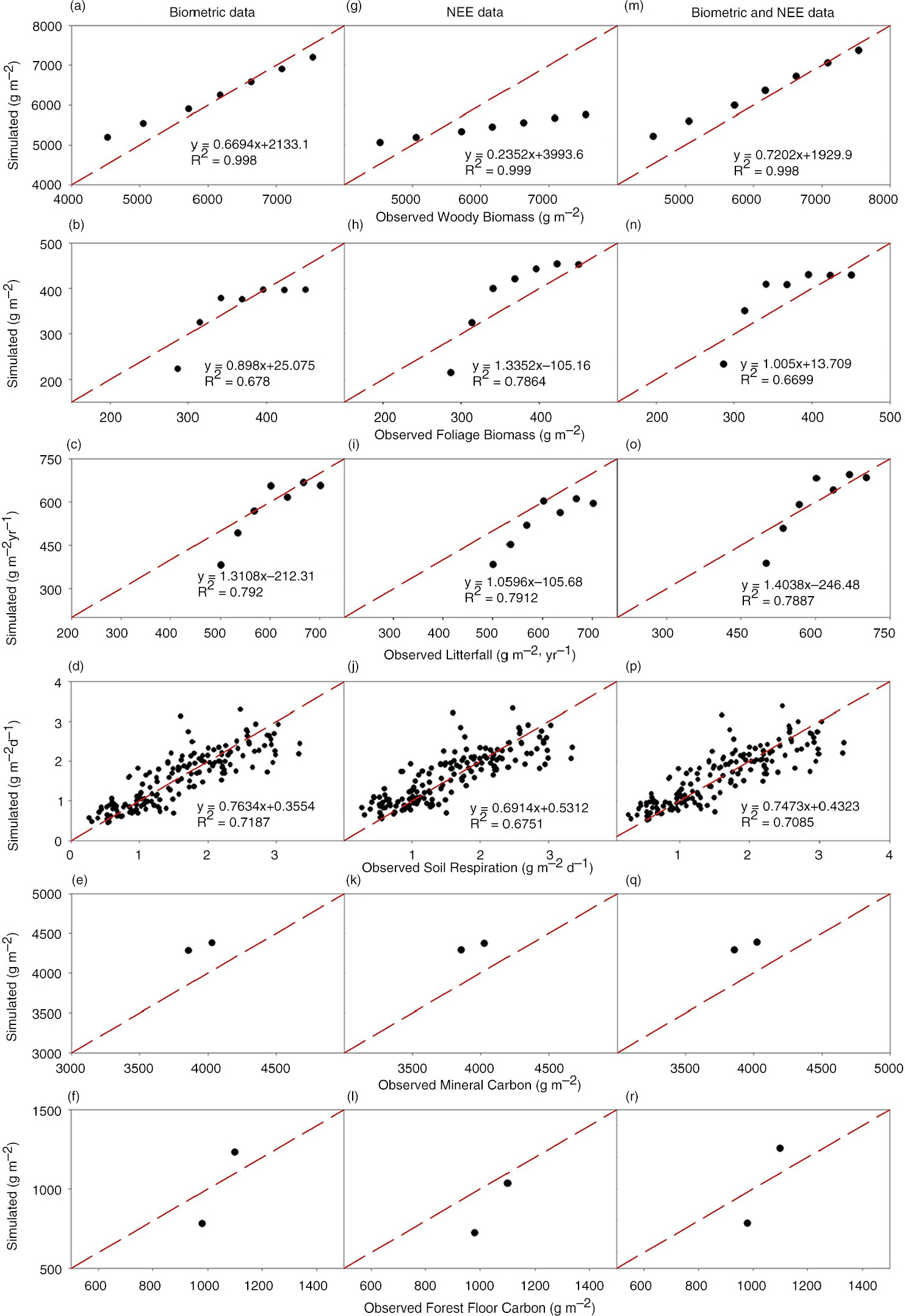
Fig. 5
Comparisons between simulated and observed woody biomass (a, g and m), foliage biomass (b, h and n), litterfall (c, i and o), soil respiration (d, j and p), mineral carbon (e, k and q), and forest floor C (f, l and r) from three experiments (NEE data, biometric data, and NEE and biometric data).
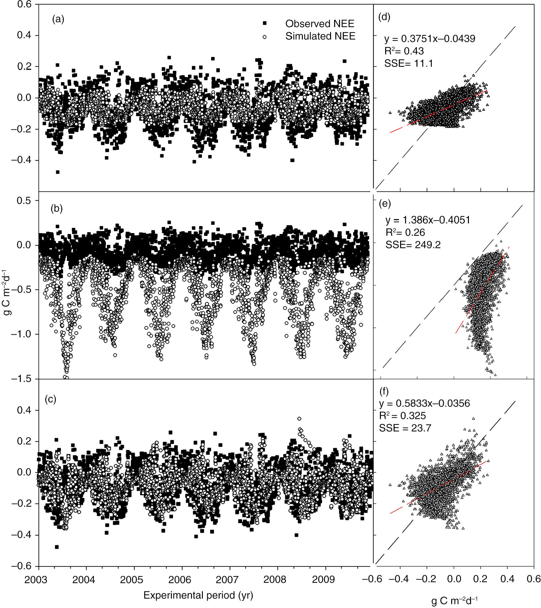
Fig. 6
Comparison of simulated and observed NEE data (from 2003 to 2010) based on three experiments (NEE data, biometric data, and NEE and biometric data combined). The simulated and observed NEE data derived from NEE data, biometric data, combined NEE and biometric data are listed in panels a, b and c; the relationships between simulated and observed NEE data are shown in panels d, e and f, respectively. SSE is sum of squares error.
3.3. Forecasting C pool sizes and its uncertainty
Forecasted C contents exhibit a greater increasing trend from 2010 to 2023 in the slow SOM (Fig. 7f) compared with that in the passive SOM (Fig. 7g). The predicted trends for woody biomass (Fig. 7a), foliage biomass (Fig. 7b), metabolic litter (Fig. 7c) and structural litter (Fig. 7d) based on Experiment 2 and Experiment 3 displayed consistencies to some extent, but differed from those on Experiment 1. The forecasted microbial C pool increased first and subsequently declined in Experiment 1, while declined first but levelled off later in Experiment 2. In Experiment 3, however, the trend increased initially and then levelled off (Fig. 7e).
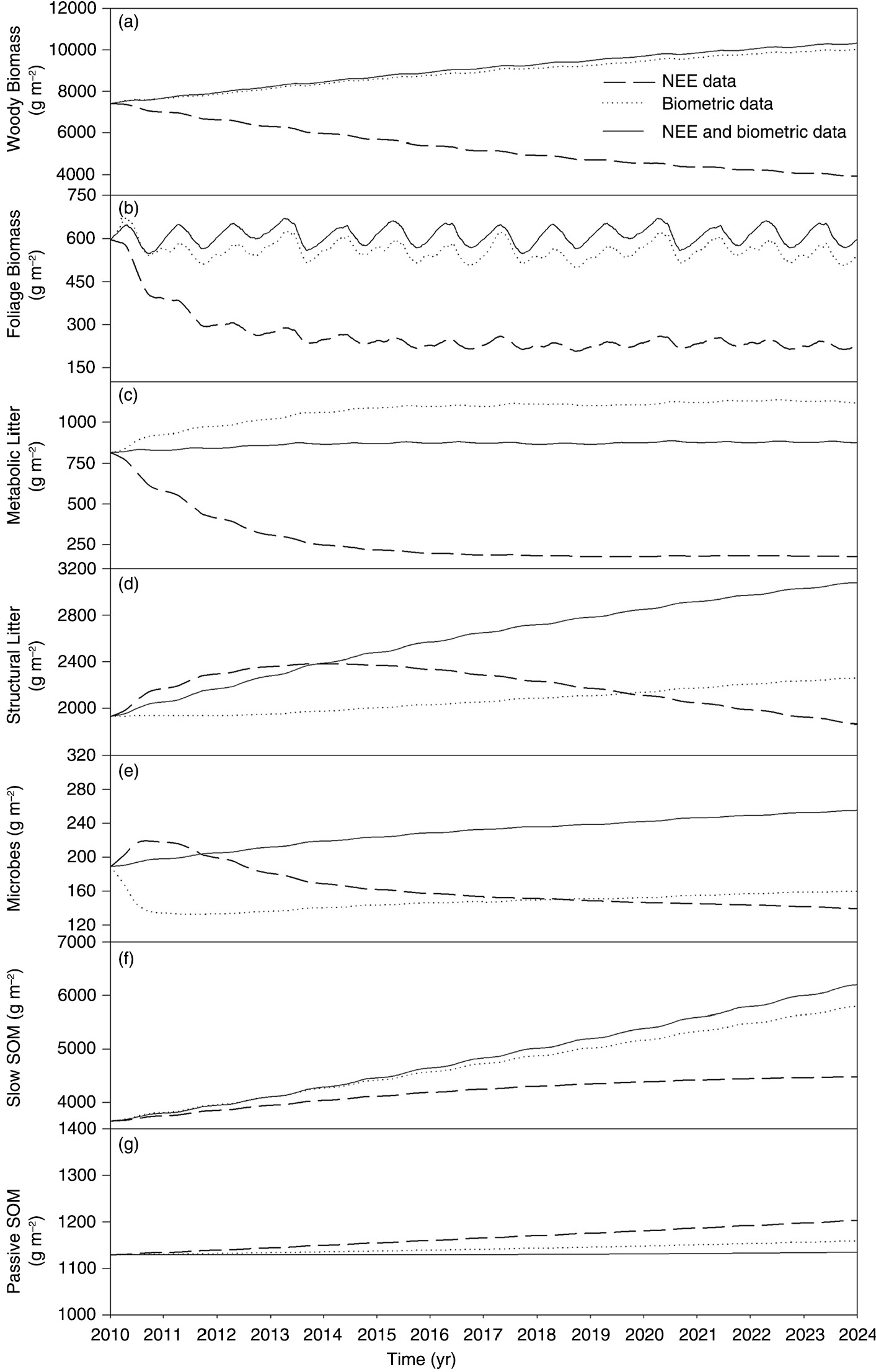
Fig. 7
Predicted woody biomass (a), foliage biomass (b), metabolic litter (c), structural litter (d), microbes (e), slow SOM (f), and passive SOM (g) from 2010 to 2023 using the parameter values of MLEs (well-constrained parameters) and means (poorly constrained parameters) from Experiment 1, 2 and 3.
In this study, we used eq. (1) with randomly selecting 100 samples from 50 000 samples to monitor the convergence of simulated C pools. Most model simulations followed the general trends of their dynamics (Fig. 8).This would be beneficial for well-constrained parameters and prior knowledge about limit intervals. The simulated C pools matched with the observed data well, especially for woody biomass, foliage biomass, litterfall and soil respiration. Among 100 samples, the scattered distribution of both forest floor C and mineral C were larger, probably due to having relatively less measured C data in the long term.
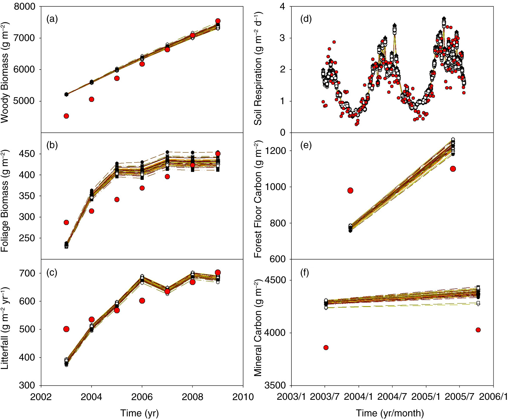
Fig. 8
C pools (i.e. woody biomass, foliage biomass, litterfall, mineral carbon and forest floor carbon) and soil respiration simulated by using 100 random parameters sampled from all 5000 parameters are listed in panels a, b, c, d, e and f. The red solid circles represent observed data and other symbols (line with point, 100 in all) represent simulated data in each panel.
4. Discussion
4.1. Complementarity of flux- and biometric-based data
The nature of inverse analysis is to exploit the information content contained in data sources, model structure and prior knowledge on parameters (Raupach et al., 2005; Xu et al., 2006). Our modified TECO model combined an ecosystem (i.e. vegetation–soil C transfer) model with a canopy photosynthesis submodel to estimate parameters from flux- and biometric-based data, which was different from previous studies directly using simulated-GPP from other models or self-loop calculated flux data as C input [e.g. the VCM GPP model in Richardson et al. (2010) and the flux data in Zhang et al. (2010)]. By conducting three experiments with different data sources (i.e. NEE data, biometric data and two combined), we found that NEE and biometric data, which were related to different processes in ecosystem C dynamics, contained complementary information in constraining parameters and further impacted the model prediction (Fig. 7).
As previous studies have reported, the different data streams may contain information of different processes involved in terrestrial C cycling (Franks et al., 1999), or of different time scales (Raupach et al., 2005; Richardson et al., 2010). The flux-based data contain considerable information on how ‘fast’ processes (NEE/GPP, soil respiration) respond to environmental drivers, while the biometric-based data mainly consist of information about relatively ‘slow’ processes (C transfer coefficients, monthly/annual dynamics of biomass, litter from wood/leaves). In our study, the NEE data mainly constrained parameters describing the processes of photosynthesis (i.e. K 25 c , E Kc and V 25 m ) and ecosystem respiration (R 0 eco ), while there were almost no constraints on C transfer coefficients (Fig. 2). NEE is a small net flux from a balance between two large fluxes of photosynthesis and respiration with a substantial amount of noise (Valentini et al., 2000; Hollinger and Richardson, 2005; Wu et al., 2009), which did not directly relate to long-term processes (i.e. C transfers). The biometric data were relatively effective in constraining C transfer coefficients from plants pools in leaves, wood and litter (Fig. 2), which supported the results from Xu et al. (2006).
The information contents from diverse data streams can help improve model parameterisation, inform the selection of model structures, analyse uncertainty of ecological forecasting and design better experiments for data collection. Previous models were usually designed and tested using data representing either only short-term processes (e.g. NEE data) or long-term processes (e.g. biometric data), mostly in a vegetation–soil C transfer model (Xu et al., 2006; Wu et al., 2009; Richardson et al., 2010). By combining the TECO model with a canopy photosynthesis model, we can contain different processes of ecosystem C dynamics (i.e. photosynthesis and ecosystem C sequestration). The complementarity of NEE and biometric data was obvious in constraining parameters (61% parameters were tightened considerably) (Fig. 2). Our results suggest that the appropriate selection of data source, which represents both short- and long-term C dynamic in a multiprocess model, can substantially reduce uncertainty in parameter estimation, and further improves model simulation (C pools and NEE, Figs. 5 and 6) and prediction (Fig. 7).
4.2. Uncertainties of parameter estimation
Use of model-data fusion for parameter estimation is one of the most common applications (Wang et al., 2009). Probabilistic inversion constructs parameter distributions and assesses parameter uncertainties by quantifying MLEs, means and confidence intervals or SDs and offers much richer information contained in the data, model structure and prior knowledge on parameters than deterministic inversion (Raupach et al., 2005; Xu et al., 2006; Zhou et al., 2010). In this study, the values of the relatively well-constrained C transfer coefficients C 1 , C 2 and C 3 in Experiment 2 and Experiment 3 are consistent with previous inversion results (Xu et al., 2006; Zhang et al., 2010). However, parameters C 4 and C 6 are lower compared with the results of Xu et al. (2006), indicating that structural litter and slow SOM turnover faster at the QYZ site, probably due to the differences in forest age and C pool size. The negative correlation between parameters C 3 and C 4 in Experiment 2 (−0.90) and Experiment 3 (−0.89) suggests that a reasonably complementary relationship exists in the C transfer rates of metabolic and structural litter, since the total litter amount was partitioned into the two pools. Although the information content contained in the biometric data is sufficient to constrain C 3 and C 4 (Fig. 4), their high correlation made separation difficult unless we have enough data on metabolic versus structural components of litter. The information contained in both NEE and biometric data was not sufficient to constrain the C transfer coefficients of microbial (C 5 ) and passive SOM (C 7 ); the lack of microbial biomass data and long-term C dynamic data are likely to be the main factors as explained by Xu et al. (2006).
To extract the information contained in the observed NEE and biometric data, our inverse analysis was performed on the basis of the TECO model structure with some limitations, particularly on the parameters for photosynthesis and soil respiration. For example, the TECO model assumes Q10 to be a constant parameter, although experimental research has shown that Q10 values always vary with temperature, moisture and/or seasons (Davidson et al., 2006). This may partially cause the uncertainties in the deviations between the predicted and observed NEE values (Fig. 6).
4.3. Model-data comparison and prediction
In our study, most model-data fitting usually had a high R 2 in C pools, especially in woody biomass (Fig. 5). However, there was still plenty of unexplained variance. The simulated woody biomass fitted the observed data poorly in Experiment 1 (Fig. 5g). In contrast to Experiment 2 and 3, the different optimal value of C 2 in Experiment 1 may be partially responsible for the differences. The systematic variation in foliage biomass was not explained by the model with parameter values constrained by NEE or biometric data or both (Fig. 5h, b and n). The reason for the discrepancy suggested by Luo et al. (2003) was the quality of the foliage biomass data, which was estimated indirectly from DBH. Direct measurements of foliage biomass would make an improvement in model fit if a suitable technique allows these measurements. Similar systematic deviations were seen in litterfall, while the main factor may be from the model structure, which may not accurately represent the processes of metabolic and structural senescence in terrestrial ecosystems.
The model-data comparison for NEE had the lowest R 2 in this probabilistic inversion (Fig. 6). The frequency and length of the available datasets may be partially responsible for the systematic deviation. Half-hourly micrometeorological data on Ta, PAR and RH were obtained from the eddy tower to simulate NEE. After using a nonlinear regression algorithm for filling gaps, there were about 120 000 values in each dataset used in this study. Another reason for the discrepancy may be from the model structure, which has some inappropriate assumptions such as those described previously about the parameter Q10.
This model incorporates information from the posterior parameter estimations (MLEs and means), the posterior correlations among parameters and the model structure into forward simulation. The micrometeorological data for the period from 2003 to 2009 were extrapolated to the 2010–2023 period by replicating the time series twice for predicting mean pool sizes (Fig. 7). The uncertainties of forward simulation are derived from the model structure itself and those unconstrained parameters (i.e. 74%, 70% and 39% of all parameters for Experiment 1, 2 and 3), in combination with the different environmental conditions. In addition, having more long-term datasets available may improve the models’ projections.
4.4. Uncertainty analysis
As an integral part of data assimilation, uncertainty analysis needs to incorporate the uncertainties in model structure, measurements, initial conditions, prior parameter values and optimisation methods (Wang et al., 2009). Our study was based on the model structure in a flux-based ecosystem submodel (FBEM) and a TECO submodel (Fig. 1), existing knowledge on the uniform prior distribution over the limit intervals (Table 1), the MCMC sampling technique and the Gelman–Rubin (G–R) diagnostic method. The FBEM and TECO submodels were designed and tested using data representing different time scales (e.g. half-hourly meteorological and NEE data in the FBEM model, interannual biometric data and diurnal soil respiration data in the TECO model). Combining the two models in this study probably led to large uncertainties. The MCMC method uses multiple datasets with 23 parameters sampled from the limit intervals and needs to run the whole model and compare all data points between the observed and simulated data. The weighing factors in eq. (4) for different datasets would vary for each instance of generating the posterior distributions of the parameters (Fig. 8). Most simulated C pools vary with time, especially foliage biomass and mineral C. We may have to explore various other setups to define the posterior PDF to improve the model's ability to match multiple datasets simultaneously.
5. Conclusion
In this study, we used an evolved TECO model by adding canopy-level photosynthesis processes and ecosystem respiration to evaluate the information content of flux- and biometric-based data in constraining terrestrial C cycle model parameters. The results showed that the NEE data mostly constrained parameters describing photosynthesis and ecosystem respiration, whereas biometric data mostly constrained C transfer coefficients among C pools. The complementarity of the two data streams was obvious when both of them were used in the model to contain different processes of terrestrial C dynamics. Such findings enhance our ability to identify information from flux and biometric data and further reduce uncertainty for parameter estimation and model prediction in terrestrial C cycle studies. Overall, our study differentiated the importance of information contents in different data streams by data assimilation with a TECO model. This knowledge is useful for model development, uncertainty analysis, future data collection and evaluation of ecological forecasting. In addition, knowledge of information contents from diverse data streams by data assimilation not only reduces uncertainty of parameter estimation and model prediction in the TECO model, but also helps accelerate our understanding of ecological processes, test ecological theory, forecast changes in ecological services and support decision making.
6. Acknowledgements
We are grateful to two anonymous reviewers and Dr. Yiqi Luo for their valuable comments and suggestions. This research was financially supported by the National Natural Science Foundation of China (Grant No. 31290221, 31370489), the Program for Professor of Special Appointment (Eastern Scholar) at Shanghai Institutions of Higher Learning, and the ‘Thousand Young Talents’ Program in China.