
1. Introduction
The energy balance of northern high-latitude permafrost regions is crucial for most ecosystem processes in Arctic land areas, including permafrost thermal conditions, plant growth, microbial activity, carbon (C) and nutrient cycling, hydrology and geomorphology. Surface energy flux dynamics is regulated by a number of factors, including available radiation, meteorological conditions, surface characteristics and soil wetness (Boike et al., 2008; Westermann et al., 2009). Arctic climate warming, which has been estimated to be almost twice as large as the global average (Christensen et al., 2007; Graversen et al., 2008) due to a phenomenon known as Artic amplification (Screen and Simmonds, 2010), will affect energy partitioning and hence the structure and functioning of Arctic terrestrial ecosystems (Hinzman et al., 2005; Post et al., 2009). Changes in Arctic energy balance partitioning may by itself induce further feedback effects on the local and global climate system (Chapin et al., 2005).
Warming in the Arctic has accelerated during recent decades (Chapin et al., 2005; Overland et al., 2008). Observations from circumpolar Arctic permafrost monitoring sites reveal increasing permafrost temperatures (Osterkamp, 2005; Åkerman and Johansson, 2008; Christiansen et al., 2010; Romanovsky et al., 2010). Dependent upon site specific conditions in permafrost and hydrological regimes increasing active layer depths (ALD) and permafrost thawing may lead to wetter (Johansson et al., 2006) or dryer (Oechel et al., 1993) soil conditions. The observed increase in shrub growth and associated increases in vegetation greenness and productivity across the circumpolar north (Beringer et al., 2005; Myers-Smith et al., 2011), affects snow dynamics, hydrologic cycle, albedo, energy and C exchange. In relation to the large amounts of soil C residing in northern high-latitude ecosystems (McGuire et al., 2009), direct and indirect effects of changes in Arctic surface energy balance are linked to potential changes in land–atmosphere exchange of greenhouse gases.
A majority of Arctic energy balance studies have been conducted in North American Arctic (e.g. Ohmura, 1982; Rouse et al., 1987, 1992, 2003; Lafleur and Rouse, 1988; Lafleur, 1992; Harazono et al., 1998; McFadden et al., 1998; Halliwell et al., 1999; Vourlitis and Oechel, 1999; Eaton et al., 2001; McFadden et al., 2003; Beringer et al., 2005; Liljedahl et al., 2011). Fewer studies have been reported from Greenland and Eurasian Arctic (e.g. Boike et al., 1998, 2008; Lloyd et al., 2001; Soegaard et al., 2001; Westermann et al., 2009; Langer et al., 2011a, 2011b). Most of these studies have been performed in wet ecosystems, whereas relatively dry ecosystems that cover vast areas of the Arctic are less well studied. In addition, most energy balance studies have focused on short periods of a summer season or a few years.
Land–atmosphere flux measurements in the Arctic are difficult to conduct; both due to the remoteness and the harsh and extreme conditions. Recent development in eddy covariance (EC) instrumentation, i.e. high frequency three-dimensional sonic anemometers and gas analysers, has enabled measurements in remote areas with little attendance. During the past decades the EC methodology (cf. Aubinet et al., 2000) has become a key tool for assessing land–atmosphere exchange of gases and energy at landscape scale, and its suitability has been demonstrated in a number of energy balance studies (e.g. Harazono et al., 1998; McFadden et al., 1998, 2003; Vourlitis and Oechel, 1999; Lloyd et al., 2001; Soegaard et al., 2001; Rouse et al., 2003; Beringer et al., 2005; Westermann et al., 2009; Langer et al., 2011a, 2011b; Liljedahl et al., 2011).
Here we present a unique 11-yr record (2000–2010) of mid-summer surface energy fluxes from a high Arctic tundra heath in Zackenberg, Northeast Greenland. We aim to describe the surface energy flux dynamics at the site and to investigate whether climatic and environmental changes such as increasing summer-time temperature and increased thaw depths in the area have caused changes in surface energy partitioning throughout the study period.
2. Materials and methods
2.1. Site description
The study area (74.47°N, 20.55°W, 38 m a.s.l.) is located in the Zackenberg valley within the Northeast (NE) Greenland National Park, between the Greenland Ice Sheet and the Greenland east coast (Fig. 1). Mountains (>1000 m a.s.l.) surround the valley to the west, east and north, while a fjord forms the southern boundary of the valley. This area has been subjected to extensive environmental monitoring activities since the mid-1990s within the auspices of Zackenberg Ecological Research Operations (ZERO). According to the climatological record at the site, the mean annual (1996–2010) temperature is −9.1°C with July being the warmest month (6.2°C) and February the coldest (−22.4°C). Annual precipitation total is 261 mm, of which approximately 85% falls as snow (Hansen et al., 2008). The Zackenberg region is characterised by continuous permafrost, and the maximum thaw depth varies between 0.4 and 0.8 m depending on soil material (Pedersen et al., 2012). Winds during winter are typically from the north (offshore), while during summer winds from southeast (onshore) dominate.
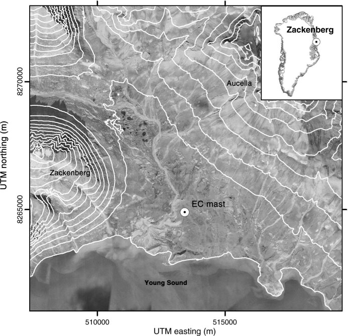
Fig. 1
Map of the study area indicating the location of eddy covariance (EC) mast (Universal Transverse Mercator (UTM) zone 27, World Geodetic System (WGS) 84). White contour lines indicate 100 m elevation intervals. Inserted map shows the location of Zackenberg in Northeast Greenland (74.47°N, 20.55°W). The average footprint of the EC system was ca. 200 m long, directed towards southeast, and dominated by Cassiope heath plant community type (Lund et al., 2012).
During 1996–2010, mean July air temperature in Zackenberg increased by 0.19°C yr−1 (p=0.016; Fig. 2a; cf. Pedersen et al., 2012). However, the interannual variability is high and as such the slope of the regression line and the significance are sensitive to the time period chosen. For the time period of this study (2000–2010), the slope is similar (0.18°C yr−1); however, the regression is not statistically significant (p=0.170). The ALD in the area represents an independent measure of the on-going environmental changes in Zackenberg. During 1997–2010 the maximum ALD has increased by 1.6 cm yr−1 (p<0.001; Fig. 2b; cf. Pedersen et al., 2012). This change is similar also for the time period 2000–2010 (slope=1.5 cm yr−1; p<0.001).
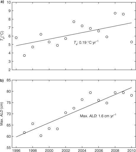
Fig. 2
Mean July air temperature (T a ) 1996–2010 (a) and maximum active layer depth (Max. ALD) 1997–2010 (b) in Zackenberg, NE Greenland.
The EC system was installed on a tundra heath, which is the dominating ecosystem type in the valley. A footprint analysis (Lund et al., 2012) revealed that the majority of the fluxes originated from within a distance of ca. 200 m, dominated by the Cassiope heath plant community type. The dominating plant species within the community, Cassiope tetragona and Salix arctica, cover approximately 31% of the Zackenberg valley (Soegaard et al., 2000), and occur throughout most of the circumpolar middle and high Arctic areas. Summer-time soil water content in the topsoil at the study site is approximately 30% while maximum leaf area index (LAI) generally ranges 0.2–0.3 (Soegaard et al., 2000).
2.2. Measurements
Fluxes of sensible (H) and latent heat (LE) were obtained from a closed path EC system. Between the years 2000 and 2007, the EC system consisted of an infrared gas analyser LI-6262 (LI-COR Inc., USA) and a 3D sonic anemometer Gill R2 (Gill Instruments Ltd, UK). Since late 2007, a LI-7000 (LI-COR Inc., USA) and a Gill R3 (Gill Instruments Ltd, UK) have been used. The anemometer was installed at a height of 3 m, and air was drawn at a rate of ca. 5.2 L min−1through ca. 7 m tubing (inner diameter: 1/8”), equipped with a 1 µm pore size filter, to the gas analyser. The H2O zero offset of the gas analyser was checked regularly, while the H2O span was calibrated retrospectively using water vapour concentrations obtained from air temperature and humidity measurements at the climate station (see below). More information on the EC system is given by Moncrieff et al. (1997), Soegaard et al. (2000) and Lund et al. (2012).
In 2000–2005, soil volumetric water content (θ v ) was measured using two ML2x ThetaProbes (Delta-T devices, UK) installed vertically immediately after snow melt in each year, providing average θ v for top 6 cm. As of 2006, ThetaProbes were installed permanently in a horizontal orientation at depths 5, 10, 30 and 50 cm. Soil heat flux (G meas) was measured between 2000 and 2007 using three heat flux plates HFP01 (Hukseflux, the Netherlands). The heat flux plates were installed in the same spot every year immediately after snow melt at a depth of 3 cm.
Approximately 150 m southwest from the EC mast, a meteorological station operated by Asiaq–Greenland Survey provided a wide range of quality checked ancillary data. Measurements of air (T a ; Vaisala, HMP 45D), surface (T s ) and soil temperature (Campbell 105T, at depths 0, 2.5, 5, 10, 20, 30, 40 and 60 cm), air humidity (Vaisala, HMP 45D), air pressure (Vaisala, PTB101B), precipitation (Precip; Ott Pluvio and Belfort, 5915 x), incoming shortwave radiation (SW in ; Kipp & Zonen CM7B) and net radiation (R n ; REBS Q*7 2000–2001, Kipp & Zonen, NR. Lite 2002–2010) were used in this study. ALD was measured manually with a steel rod in a nearby active layer monitoring area (100*100 m, 11*11 grid points), ZEROCALM-1 (Circumpolar Active Layer Monitoring-Network-II), in biweekly intervals.
2.3. Turbulent fluxes
Data from the EC system were acquired from the analysers’ digital-to-analogue converters, aligned to anemometer data, and collected on a computer running Edisol software (Moncrieff et al., 1997). Raw data files were processed in EdiRe software (Robert Clement, University of Edinburgh) and sensible (H) and latent heat fluxes (LE) were calculated on a 30 minutes basis. The processing list included despiking (Højstrup, 1993), 2-D coordinate rotation, time lag removal between anemometer and gas analyser data by covariance optimisation, correction for humidity effects on sonic temperature, block averaging, frequency response corrections based on model spectra and transfer functions (Moore, 1986), and WPL correction (Webb et al., 1980). Flux data was screened for low friction velocity (u *<0.1 m s−1). This threshold, which is often used in EC studies (Gu et al., 2005), was chosen to avoid situations with strongly stable conditions during which the EC methodology may fail to capture the fluxes of H and LE. Fluxes of LE and H were quality checked using monthly 2nd order polynomial fits with R n (Ohta et al., 2008). Outliers at a distance of more than three standard deviations from the model were excluded (excluded on average 2.5±0.5% and 2.6±0.5% of H and LE data, respectively, in each year). No gap-filling was performed as the focus of this study was on energy flux ratios and bulk parameters;, thus only original, measured and quality checked H and LE data were used in subsequent analyses.
2.4. Soil heat flux calculations
The soil heat flux at the surface (G meas, sur) was calculated by adding the energy stored (S, W m−2) above the heat flux plates (Mayocchi and Bristow, 1995) to the measured flux (G meas):
where ΔT s /Δt is change in soil temperature (K) with time t (s) at soil heat flux plate installation depth d (m), and C s is soil heat capacity (J m−3 K−1), calculated as:
where ρ b is bulk density (900 kg m−3, Elberling et al., 2008), C d is dry soil heat capacity (840 J kg−1 K−1, Hanks and Ashcroft, 1980), θ v is volumetric soil water content (m3 m−3), ρ w is water density (1000 kg m−3) and C w is water heat capacity (4186 J kg−1 K−1).
2.5. Data analyses
All analyses were performed on midday (11:00 – 15:00 local time) data from the mid-summer period in each year. Mid-summer period was, based on Weller and Holmgren (1974) and Dingman et al. (1980), defined as the period with daily average air and top soil temperatures above 0°C, positive SW in and R n , and albedo between 10 and 20%. All ratios and variables were screened for extreme amplitudes (values outside mean±3 standard deviations), before calculating daily averages.
The mid-summer period energy balance of the Zackenberg heath tundra surface can be defined as:
When directed away from the surface, H, LE, and G are positive. For a vegetation covered surface, an additional storage term could be included in the energy balance equation; however, due to the sparse and slender vegetation cover in the Zackenberg heath, this term has not been considered in this study. Likewise, the energy consumed in photosynthesis is considered negligible. In order to investigate the relative magnitude of H, LE and G in the surface energy balance [eq. (3)], i.e. the partitioning of total available energy at the surface, ratios of H/R n , LE/R n and G/R n were calculated. Furthermore, the Bowen ratio (β=H/LE) was calculated, describing the type of convective heat loss (sensible vs. latent heat) from the surface. In general, wet surfaces are expected to have lower β compared with dry surfaces (Eaton et al., 2001).
The soil heat flux (G) was modelled in order to provide a consistent data set throughout the study period (Halliwell and Rouse, 1987):
where T o −T 2.5 is temperature difference between surface and 2.5 cm depth and ɛ is a scaling parameter. Between 2000 and 2007, ɛ was optimised using non-linear least squares regression with G meas, sur and as dependent (y) and independent (x) variables, respectively (y=b 0x+b 1; b 0=1.03±0.04, b 1=−2.28±3.4, r 2=0.82±0.23). Obtained values of ɛ were in the range 0.28–0.51, with a significant decreasing trend between 2000 and 2007 (−0.028 yr−1, r 2=0.74, p=0.013). The systematic deviation from ɛ=1 may be explained by radiation absorption of the Campbell 105T sensor being higher than for the soil, and also a possible overestimation of C s and/or ρ b C d . For 2008–2010, when no G meas was available, the observed decrease in ɛ was extrapolated resulting in values of 0.29±0.10, 0.26±0.11 and 0.23±0.12, respectively, and used for modelling G. As this method is not reliable during phase change of water, modelling G was confined to periods of time with thaw depth>10 cm.
In order to study the dynamics of the surface (including both soil and vegetation) in terms of its evapotranspirative characteristics, the surface resistance (r s , s m−1) was calculated by inverting the Penman-Monteith equation (Shuttleworth, 2007):
where Δ is slope of the saturated vapour pressure curve (Pa K−1), γ is psychrometric constant (Pa K−1), ρ is density of air (kg m−3), c p is specific heat capacity of air at constant pressure (J kg−1 K−1), D a is atmospheric vapour pressure deficit (Pa) and A is energy available for evapotranspiration (W m−2). In this study, A is equated as the sum of H and LE. The surface resistance describes the control of latent heat transfer by plants and bare ground.
The aerodynamic resistance (r a , s m−1), describing the role of atmospheric turbulence for water vapour and sensible heat transfer, was defined as (Monteith and Unsworth, 1990):
where u is wind speed (m s−1) and u * is friction velocity (m s−1) obtained from the EC measurements. To describe the relative importance of r s and r a , the McNaughton & Jarvis Ω value was calculated (Jarvis and McNaughton, 1986):
Low values of Ω (r s >> r a ) indicate that D a is main driver of evapotranspiration (i.e. physiological control), while Ω values approaching 1 indicate dominant control by available energy (R n ). Furthermore, the Priestley-Taylor coefficient α (Priestley and Taylor, 1972) was calculated as:
The α coefficient varies in space and time according to surface type and meteorological conditions. Values of α are approximately 1.26 in areas where vegetation cover is complete and of short stature and where the surface is well supplied with water (Priestley and Taylor, 1972). In the Arctic, α values are generally found to be below 1.26. In an extensive review covering the Arctic domain, Eugster et al. (2000) reported α values ranging from 0.54 to 1.51, where higher values were characteristic for wet, lowland areas whereas lower values were typical for dry, upland areas.
To evaluate the importance of surface wetness for the energy flux dynamics, the surface saturation vapour pressure deficit (D s ) was calculated (Eaton et al., 2001):
where e so is surface saturation vapour pressure (Pa) and e o is actual surface vapour pressure (Pa). The deficit D s describes how close the thin (ca. 1 cm) layer of air immediately above the surface is to saturation (Eaton et al. 2001). The variable e so is modelled from surface temperature (T o in °C) according to Campbell and Norman (1998):
Similar to Eaton et al. (2001), e o is derived from:
where e a is atmospheric vapour pressure (Pa) and T a is air temperature (°C).
3. Results and discussion
The mid-summer periods during 2000–2010 in Zackenberg, NE Greenland, lasted on average between DOY 167±7 and 244±7 (16 June – 1 September for a non-leap year), with an average length of 78±9 d (Table 1). There were no significant trends in timing of start, end or length of mid-summer period (Table 1). The timing of onset of mid-summer period correlated significantly with DOY of snowmelt (p<0.001). On average, the mid-summer period began 2 d following DOY of snowmelt.
Table 1. Mid-summer period surface energy balance and environmental characteristics during the study period 2000–2010
The extensive data set on surface energy balance components and supporting meteorological and soil physical characteristics from Zackenberg, NE Greenland (2000–2010), allowed us to describe an average year mid-summer period for the high Arctic tundra heath site (Fig. 3). This period was generally characterised by decreasing levels of net radiation (R n ), increasing air temperature (T a ) and decreasing volumetric soil water content (θ v ). During the first few days following snow melt, soil heat flux (G) was high; consuming ca. 30% of the available energy, related to the steep temperature gradient between surface and permafrost table (Rouse, 1984; Langer et al., 2011a). Energy partitioning into latent heat fluxes (LE/R n ) peaked after approximately 1 week when θ v was still relatively high. After approximately 2 weeks, the ratio of sensible heat flux (H) to R n , reached ca. 55%, a level that was mostly maintained during the remainder of the average year mid-summer period. Thus, similar to the findings by Boike et al. (1998) at a Siberian tundra site, H was the dominant heat sink during the mid-summer period, except for the first 1–2 weeks when thin active layer and high θ v allowed for high energy partitioning into G and LE.
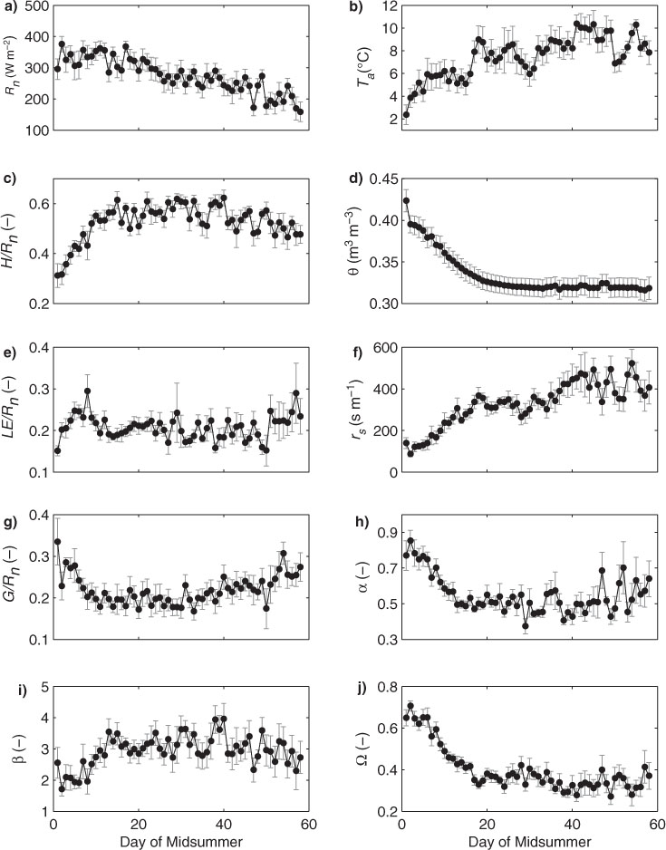
Fig. 3
Environmental characteristics and surface energy dynamics during average year mid-summer period. (a) net radiation (R n ); (b) air temperature (T a ); (c) ratio of sensible heat (H) to R n ; (d) soil volumetric water content (θ v ); (e) ratio of latent heat (LE) to R n ; (f) surface resistance (r s ); (g) ratio of ground heat flux (G) to R n ; (h) Priestley-Taylor α coefficient; (i) Bowen ratio (β); and (j) McNaughton & Jarvis Ω value. Black dots represent means and error bars standard error. Mid-summer period is defined as the period with daily average T a and T 0 above 0°C, positive SW in and R n , and albedo between 10 and 20%. Mean start and end dates during the study period (2000–2010) were 16 June and 1 September, respectively.
The Bowen ratio (β) was relatively low (ca. 2) during the first week (Fig. 3), whereas after 2 weeks it was generally varying around 3. This pattern can be explained by high surface wetness during early mid-summer period allowing for high rates of evaporation. Other studies have reported decreasing β as vascular plants develop and start to transpire water and thus contributing to LE (Lloyd et al., 2001; Boike et al., 2008). In our average year data (Fig. 3), such trend in β is not apparent. However, the generally increasing trend in surface resistance (r s ) halted between the days of mid-summer 18–35, which could be attributed to vascular plant transpiration activity. Indeed, maximum carbon dioxide (CO2) uptake during 2000–2010 in the Zackenberg heath occurred on average 32±11 d after snowmelt (Lund et al., 2012). The weak vegetation signal in this study can be ascribed to tender vegetation with low biomass residing at the site (maximum LAI ca. 0.3; Soegaard et al., 2001). Generally, for Arctic ecosystems with low vascular plant cover, a majority of evapotranspiration (55–90%) is represented by evaporation (Dingman et al., 1980; Engstrom et al., 2006), and the Zackenberg heath is likely found at the higher end of that range.
The Priestley-Taylor α coefficient was highest immediately following snowmelt when θ v was high (Fig. 3); however, it was generally below one indicating that evapotranspiration did on average not reach its potential rate (i.e. α=1.26; Priestley and Taylor, 1972). Again, this demonstrates the importance of evaporation for the LE signal, and the low transpiration activity of the resident plant community on the Zackenberg heath restraining LE fluxes. The McNaughton & Jarvis Ω value showed a similar pattern as α, indicating that for an average year R n had dominant control on LE during the first 1–2 weeks into the mid-summer period. As the soil dried out, Ω generally fell below 0.4, indicating that the importance of atmospheric vapour pressure deficit (D a ) as a controlling factor for LE increased.
The relative importance of R n and D a for surface energy partitioning demonstrated some interesting features of the Zackenberg heath. Within individual years, β generally increased with increasing R n until levels of ca. 300 W m−2, after which it in some years slightly decreased again (exemplified by year 2003 in Fig. 4). The decrease in β at the high end of R n range can be assigned to the fact that maximum levels of R n generally occurred during early mid-summer period when θ v was high (Fig. 3), allowing for high LE. The observed relationship between β and D a indicates that at low D a , a large fraction of available energy was partitioned into H. However, at increasing D a , β generally decreased (Fig. 4). Thus, the capacity of the atmosphere to hold additional water vapour was an important factor controlling surface energy partitioning. Also, β generally showed a response to changes in surface saturation vapour pressure deficit (D s ; Fig. 4). When D s was low, indicating that the surface boundary layer was close to being saturated, β was also low. Indeed, throughout the study period, besides β, D s was found to have within-year couplings also to Ω, α and r s ; especially in the range 0–500 Pa where Ω, α and r s generally responded linearly to changes in D s (exemplified by year 2007 in Fig. 5). Compared with θ v , D s reacted immediately to rainfall events increasing surface wetness (data not shown). Eaton et al. (2001) assessed whether D s could describe spatial variation between various Arctic surface and ecosystem types such as lakes, wetlands, tundra and forest. No clear relationship was found, although wet sites with high evapotranspiration rates generally had lower D s compared with dry sites. Here, we demonstrate the usability of D s for describing within-year temporal variation in surface energy dynamics at a high Arctic heath. However, as D s relates to ground surface level conditions, its applicability may be reduced in ecosystems with high and more dense canopies such as shrub tundra and wooded areas.
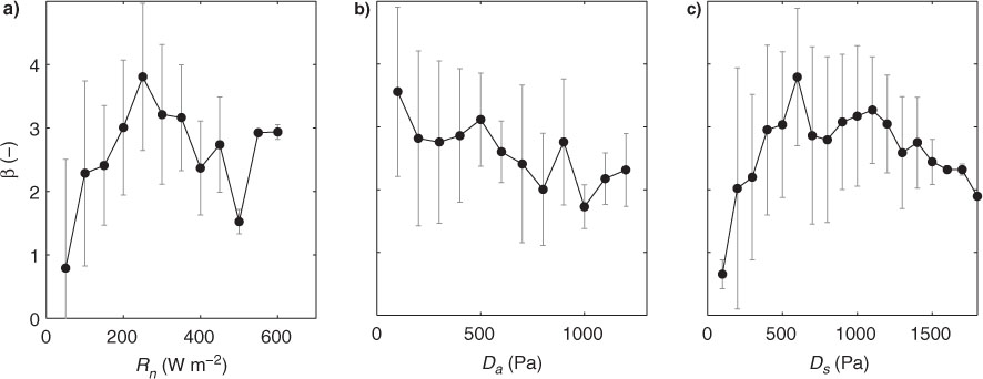
Fig. 4
Relationship between within-year variations in Bowen ratio (β) and environmental characteristics during 2003. (a) net radiation (R n ); (b) atmospheric vapour pressure deficit (D a ); and (c) surface saturation vapour pressure deficit (D s ). Observations of β was averaged within bins of 50 W m−2 (R n ) and 100 Pa (D a , D s ), respectively. Black dots represent means and error bars standard deviation.
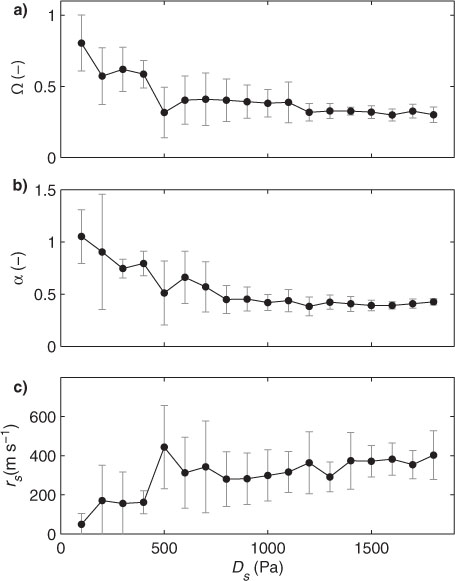
Fig. 5
Relationship between surface saturation vapour pressure deficit (D s ) and environmental characteristics during 2007. (a) McNaughton & Jarvis Ω value; (b) Priestley-Taylor α coefficient; and (c) surface resistance (r s ). Observations of Ω, α and r s was averaged within D s bins of 100 Pa. Black dots represent means and error bars standard deviation.
Several authors have stressed the importance of onshore vs. offshore winds for surface energy balance dynamics (e.g. Rouse, 1984, Lafleur and Rouse, 1988; Weick and Rouse, 1991; Harazono et al., 1998; Eugster et al., 2000). In Zackenberg, south-easterly winds typically dominate during summer (Hansen et al., 2008), thus, the local summer-time climate at the site is dominated by onshore winds carrying cold and moist air (Fig. 1). More specifically, compared with offshore winds, onshore winds (here defined as winds from 45 to 225° relative to north) in Zackenberg were characterised by lower T a and D a , resulting in higher H/R n and lower LE/R n and consequently higher β (exemplified by year 2002 in Table 2). In some years (2000, 2002, 2004 and 2006), G/R n was significantly lower for onshore compared with offshore winds. Also, α was generally lower and r a and r s generally higher during onshore wind conditions. In northern coastal zones, onshore winds bring cold, moisture-laden air masses over land resulting in steep surface-air temperature gradients and low D a resulting in enhanced H/R n and suppressed LE/R n (Eugster et al., 2000). We thus hypothesise that the local climatic conditions together with low transpiration activity of the slender vegetation and the relatively (to other Arctic study sites) dry soil conditions, bear responsibility for the observed high values of H/R n and β, and low values of LE/R n compared with other sites.
Table 2. Average midday, mid-summer meteorological conditions and surface energy partitioning characteristics during 2002 (means±standard deviation)
The energy balance closure was on average 95% (Table 1), ranging between 87% (2008) and 107% (2003). Insufficient energy balance closure is generally explained by instrumental and methodological uncertainties, insufficient estimations of storage terms, and unrepresentativeness of point scale G estimations compared with R n and eddy flux measurements of H and LE that are averaged over a larger area (Wilson et al., 2002; Foken, 2008). Correcting the unclosed energy balance artificially by allocating the residual to H and LE according to β (Twine et al., 2000), may introduce further errors as it cannot be confirmed with certainty that the reason for lack of energy balance closure lies solely within fluxes of H and LE, nor that H and LE should be equally affected by measurement limitations due to differences in sensors for measuring temperature and humidity (Foken, 2008). Measurements of R n using Q*7 and NR. Lite have an associated uncertainty of about 20% (Foken, 2008; Langer et al., 2011a); thus, the observed energy balance closure term in this study is within the uncertainty range of R n measurements. The uncertainty of turbulent fluxes (H and LE) measured with the EC method generally ranges 10–20%, dependent on the applied quality control schemes (Mauder et al., 2006). In this study, flux measurements were performed in a nearly ideal location with flat, homogeneous terrain>500 m surrounding the EC mast. A footprint analysis revealed that fluxes on average emanated from within ca. 200 m from the southeast, dominated by the Cassiope heath plant community type (Lund et al., 2012). Only midday values with u * >0.1 m s−1 were considered; thus, problems related to insufficient atmospheric mixing can be considered minimal. It should be noted that energy stored in vegetation and consumed in plant photosynthetic activity was not considered, due to the tender vegetation with low biomass residing in the Zackenberg heath. Highest uncertainty in this study is related to G estimation. A simple model based on surface and soil temperature was used to estimate G [eq. (4)]. Information on bulk density and soil heat capacity, which are spatially variable due to variations in soil moisture, texture and organic content and periglacial processes (e.g. cryoturbation), was derived from literature. Although the model performed well compared with actual soil heat flux measurements (G meas, sur) during 2000–2007, its performance during 2008–2010 cannot be validated (extrapolation uncertainty for 2008–2010 is shown in Fig. 6). However, calculating a residual term from Rn-(H + LE) can perform an independent assessment of G throughout the study period. Such proxy for G, although inheriting the uncertainties related to measurements of R n and convective fluxes, displays a similar significant trend as modelled G (Fig. 6). Overall, the observed energy balance closure in this study is in the upper range of closures reported for carefully designed experiments (Wilson et al., 2002; Foken, 2008). As such, we are confident that the energy balance components in this study are satisfactorily represented. Since the same methods were used throughout the study period, possible minor biases cannot be expected to have large effects on the observed changes.
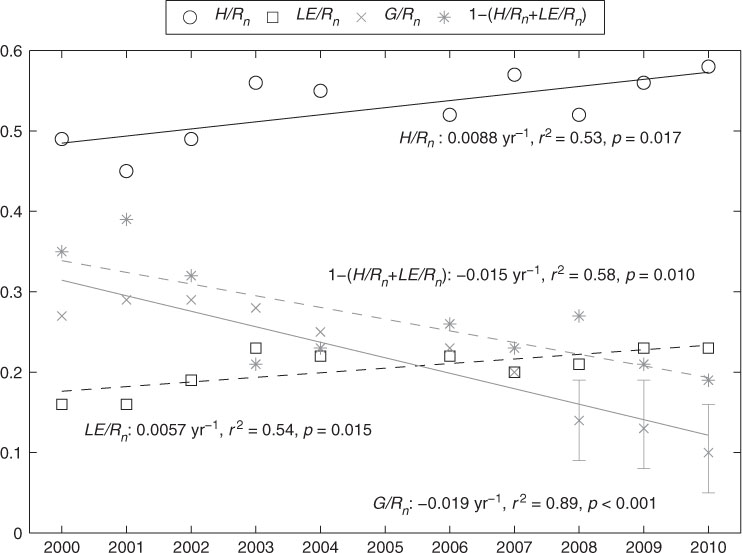
Fig. 6
Changes in mid-summer surface energy balance partitioning between 2000 and 2010. Lines indicate significant change in data. Error bars for G/R n 2008–2010 indicates uncertainty (St. dev.) in extrapolating ɛ [eq. (4)]. 1-(H/R n +LE/R n ) is a residual term in the energy balance serving as an independent proxy for G. Mid-summer period is defined as the period with daily average T a and T 0 above 0°C, positive SW in and R n , and albedo between 10 and 20%.
Fluxes of H, LE and G constituted on average 53, 20 and 22% of R n during mid-summer periods 2000–2010 (Table 1). Compared with other Arctic sites (Eugster et al., 2000; Eaton et al., 2001; Boike et al., 2008; Westermann et al., 2009; Langer et al., 2011a; Liljedahl et al., 2011), H/R n and G/R n are generally high while LE/R n is low. Consequently, average β in this study is comparably high. However, most previous studies have been conducted in wet ecosystems, where high evapotranspiration rates can be expected (Eugster et al., 2000). McFadden et al. (1998) studied energy balance partitioning over five tundra vegetation types in Arctic Alaska, and found highest β at a heath site (2.25) and lowest β at a wet sedge tundra site (0.37). In a wet polygonal tundra in Siberia, β and G/R n was 1.29 and 0.29 in a dry year, respectively, whereas in a wet year, these ratios were reduced to 0.36 and 0.17, respectively (Boike et al., 2008). Similarly, Liljedahl et al. (2011) reported higher average midday summer-time β in a dry year (1.79±0.25) compared with a wet year (1.33±0.32) for an Arctic coastal wetland in Alaska.
Average environmental conditions during the mid-summer periods 2000–2010 indicate no significant changes across years in air and soil temperatures (Table 1), despite that average July air temperatures between 1996 and 2010 in Zackenberg have increased with 0.19°C yr−1 (Fig. 2a). This can be assigned to the high inherent natural variability of the climate system and also the definition of mid-summer period in the present study, resulting in varying timing of onset and end of mid-summer period between years. Nor were there any significant changes in precipitation or SW in (Table 1). However, θ v decreased (−0.010 m3 m−3 yr−1; r 2=0.78, p<0.001) and maximum active layer depth (max. ALD) increased (1.5 cm yr−1; r 2=0.73, p<0.001) significantly. Significant linear changes (p<0.05) in surface energy dynamics during the study period were found for H/R n , LE/R n , G/R n , β and Ω (Table 1, Fig. 6). H/R n and LE/R n increased at a rate of 0.0088 yr−1 and 0.0057 yr−1, respectively, while G/R n decreased at a rate of −0.019 yr−1. At the same time, β decreased (−0.071 yr−1) and Ω increased (0.005 yr−1). It is interesting to notice that if the residual from the energy balance closure is used to correct H/R n and LE/R n according to β (Twine et al., 2000), changes in H/R n and LE/R n are further strengthened. Energy balance closure corrected H/R n and LE/R n increased at a rate of 0.0119 yr−1 (r 2 =0.72, p=0.002) and 0.0073 yr−1 (r 2 =0.88, p=0.001), respectively (data not shown).
Interannual variation in H/R n , LE/R n , G/R n and β, respectively, correlated significantly with max. ALD. In addition, G/R n , as well as Ω, correlated significantly with θ v . In areas with permafrost, a substantial amount of available energy at the surface is used to increase the active layer depth. This energy cannot be used to increase surface temperatures, constituting a negative feedback effect from thawing active layer to surface and soil temperatures (Rouse, 1984; Eugster et al., 2000; Langer et al., 2011a). However, as the active layer deepens, which is the case in Zackenberg were maximum thaw depths have increased by 1.6 cm yr−1 (Fig. 2b), this controlling mechanism is reduced. In many areas across the circumpolar north, an increased vegetation greening and productivity have been observed (Myers-Smith et al., 2011); such changes are likely to lead to increased evapotranspiration rates (Chapin et al., 2005). In Zackenberg, however, a greening trend has not been observed yet (Schmidt et al., 2012).
A change in Arctic land surface energy partitioning increasing turbulent heat fluxes will act to warm the atmosphere, thus constituting a positive feedback on the climate system contributing to Arctic amplification. Increased partitioning of R n into H is a direct pathway to warm the atmospheric boundary layer (Eugster et al., 2000), whereas for LE, the picture is less obvious. Locally, increased evapotranspiration leads to cooling. However, over larger geographical scales increased atmospheric water vapour content is likely to increase warming (Eugster et al., 2000; Callaghan et al., 2011). A positive feedback effect from changes in surface energy balance on the climate system (increased local to regional air temperature) may increase Arctic CO2 and CH4 emissions, as they are generally found to respond positively to changes in temperature (cf. Christensen et al., 2003; McGuire et al., 2009; Parmentier et al., 2013).
Continued global warming will lead to further changes in the Zackenberg region (Stendel et al., 2008) as well as in the Arctic as a whole (Christensen et al., 2007). At the end of this century, large changes are expected along the east coast of Greenland, where positive degree days will become the rule. Precipitation will increase, resulting in intensified hydrological cycle with increased winter time snow depth and more specific humidity in the atmosphere (Stendel et al., 2008). The accelerated rate of sea ice decline (Overland et al., 2011; Parmentier et al., 2013) poses a strong feedback effect on Arctic climate, however, the effect on tropospheric temperature is mainly during autumn and winter, when the heat stored in the Arctic Ocean is released to the atmosphere (Overland and Wang, 2010; Screen and Simmonds, 2010; Overland et al., 2011; Serreze and Barry, 2011). During summer, direct radiative forcing from greenhouse gases has been found to be the primary factor for tropospheric warming in the Arctic (Screen et al., 2012). Changes in atmospheric circulation as a result of global warming and Arctic amplification processes have been observed, such as the enhancement of the so-called Arctic Dipole (AD) since 2007, which has led to increased meridional flow across the Arctic accelerating sea ice loss and promoting continued warming (Overland and Wang, 2010; Overland et al., 2012). Future changes in atmospheric circulation can be expected, however, the effect on Arctic climate is yet to be understood (Serreze and Barry, 2011; Overland et al., 2012). Taken together, the predicted changes, most importantly higher temperature and prolonged thawing season, will further promote permafrost thaw and increased ALD and thus act to strengthen the observed changes in summer-time surface energy partitioning in this study.
4. Summary and conclusions
Regional and local climate are strongly influenced by surface energy partitioning (Eugster et al., 2000), and changes in energy balance partitioning may feedback on the climate system (Chapin et al., 2005). In this study, using an extensive data set from a high Arctic heath site in Zackenberg, NE Greenland, we observed an increased partitioning of available energy into H and LE, and decreased partitioning into G, between 2000 and 2010. The observed environmental changes at this site including increases in mean July temperature and active layer depth and decrease in soil wetness, have resulted in increased turbulent heat fluxes into the atmospheric boundary layer. In order to assess the effect of changes related to surface energy balance across the Arctic, more long-term data sets are needed, and obtaining such constitutes an important area for future research. The most important findings in the present study for the surface energy dynamics in Zackenberg heath include:
Summer-time local climatic conditions dominated by onshore winds carrying cold and moist air, slender vegetation with low transpiration activity and relatively dry soils; caused the observed high H/R n and β, and low LE/R n .
We demonstrated the usability of surface saturation vapour pressure deficit (D s ) for explaining within-year temporal variation in surface energy exchange partitioning.
Between 2000 and 2010, we observed increased H/R n and LE/R n , and decreased β and G/R n , associated with increasing active layer depth.
More long-term data sets on surface energy balance dynamics for various Arctic ecosystems are urgently needed to assess the impact of the observed and predicted changes across the Arctic.
5. Acknowledgements
The authors wish to thank the GeoBasis program for running the flux measurement systems, ClimateBasis program for meteorological observations, and Zackenberg Ecological Research Operations for logistical support. This study was made possible through a generous grant from the Danish Energy Agency.