
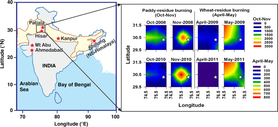
Fig. 1
Map of study locations: Patiala, Hisar and Kanpur in the Indo-Gangetic Plain (shown as yellow shaded area), at Barapani near Shillong in NE-Himalaya and at Ahmedabad and Mt Abu in semi-arid western India. MODIS derived fire-counts (plotted on the right) during the paddy- and wheat-residue burning period in the source region; sampling site at Patiala (shown by open star) is located downwind of major field-fires.
{ label needed for table-wrap[@id='UT0001'] }
Table 1. Concentrations of carbonaceous species and characteristic ratios (Av±sd given in parenthesis) from biomass burning emissions and fossil-fuel combustion in the Indo-Gangetic Plain (IGP)
[ii] bCorrelation analysis. S (significant difference for p<0.05) and IS (insignificant difference for p>0.05).
[iii] ΣPAHs (PM2.5-bound) include: NAPH, naphthalene; ACY, acenaphthylene; 2-BrNAPH, 2-bromonaphthalene; ACE, acenaphthene; FLU, fluorene; PHEN, phenanthrene; ANTH, anthracene; FLA, fluoranthene; PYR, pyrene; BaA, benzo[a]anthracene; CHRY+TRIPH, chrysene/triphenylene; B[b,j,k]FLA, benzo[b+j+k]fluoranthene; BaP, benzo[a]pyrene; IcdP, indeno[1,2,3-cd]pyrene; D[ah,ac]ANTH, dibenzo[a,h+a,c]anthracene}; BghiP, benzo[g,h,i]perylene.
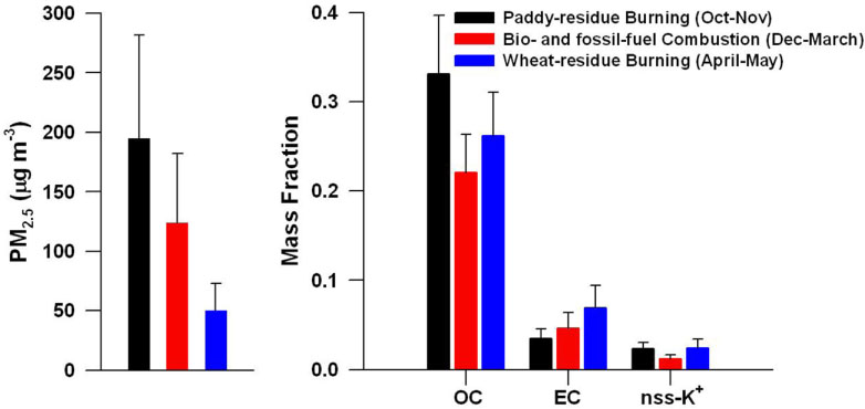
Fig. 2
Temporal variability in PM2.5 and mass fractions of OC, EC and nss-K+ associated with different emissions from source region (Patiala, Fig. 1) in the Indo-Gangetic Plain. The nss-K+=K+ aerosol – 0.037*Na+ aerosol; where K+/Na+ mass ratio of 0.037 is used for sea-salt contribution of K+ (Keene et al., 1986).
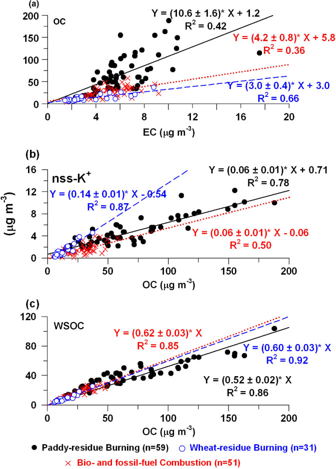
Fig. 3
Scatter plots of (a) EC vs. OC; (b) OC vs. non-sea-salt: nss-K+; and (c) OC vs. WSOC during different emissions in the IGP.
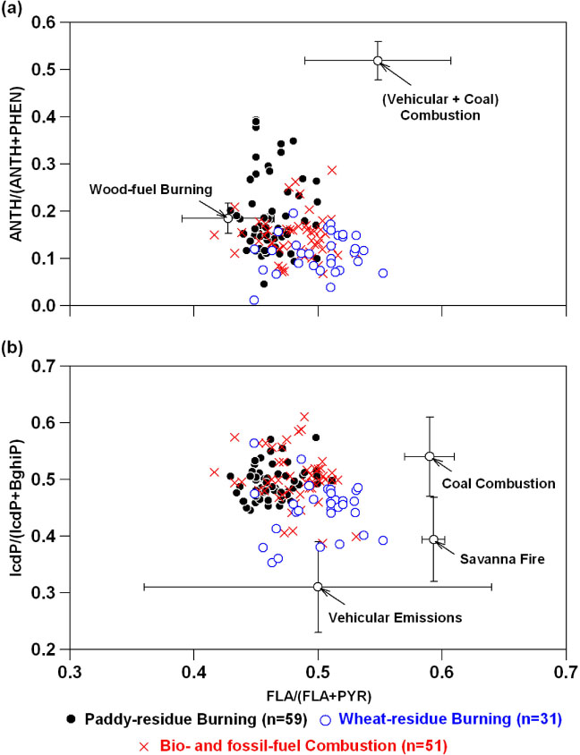
Fig. 4
Cross plots of PAH isomers showing distinct differences for the biomass burning emission vis-à-vis fossil-fuel combustion in the IGP: (a) FLA/(FLA+PYR; 4-ring on X-axis) vs. ANTH/(ANTH+PHEN; 3-ring on Y-axis); and (b) FLA/(FLA+PYR; 4-ring on X-axis) vs. IcdP/(IcdP+BghiP; 6-ring on Y-axis). Other data source: wood-fuel burning (Bari et al., 2009); (Vehicular+Coal) combustion (Sharma et al., 2008); vehicular emission (Khillare et al., 2005a, b; Rajput and Lakhani, 2008); coal combustion (Kirton et al., 1991; Khalili et al., 1995; Li et al., 2010); savanna fire (Masclet et al., 1995).
Table 2. Spatial distribution of OC/EC ratio in ambient aerosols from the Indo-Gangetic Plain (IGP) and different locations during wintertime (December–March)
Table 3. Emission budget of carbonaceous species from post-harvest agricultural-waste burning in the Indo-Gangetic Plain (IGP)
(g/kg)Fuel loadb
(Kg/sq. km)Area burntc
(sq. km/y) Emission budgetdOC7.6±1.211.8×10548 400436±68 Gg/yEC0.72±0.0341±2 Gg/yΣPAHs2.8±0.5e161±31 Mg/yWheat-residue burning (April–May)OC1.2±0.035.94×10548 40069±2 Gg/yEC0.31±0.0218±1 Gg/yΣPAHs0.4±0.1e21±6 Mg/y
[i] aEF modified, after (Kanokkanjana et al., 2011) for paddy-residue burning and, after (Hays et al., 2005) for wheat-residue burning.
[ii] bAdopted from a study in the IGP (Badarinath et al., 2006).
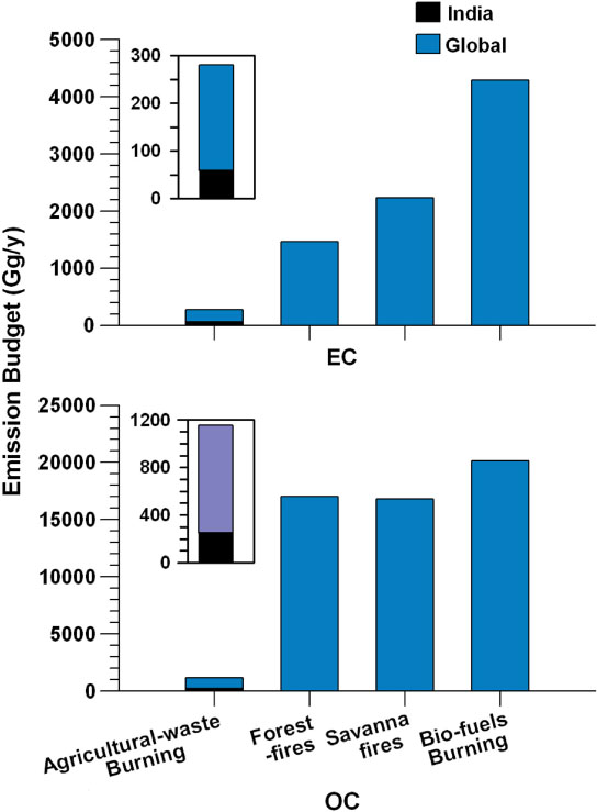
Fig. 5
Emission budgets of aerosol OC (primary) and EC from different biomass burning over the globe. Our data put together with a recent emission inventory suggest that OC and EC produced from agricultural-waste burning in the IGP (Northern India; shown as inset) contributes to ~22% [primary OC: 252±34 Gg/y] and 21% [EC: 59±2 Gg/y], respectively, on the global agricultural-waste burning emission scale.