Characteristics and emission budget of carbonaceous species from post-harvest agricultural-waste burning in source region of the Indo-Gangetic Plain

2.1. Sampling site description

The large-scale biomass burning emission in Northern India (mainly in Punjab, Haryana and western Uttar Pradesh; 2°×2°=48400 sq km; Fig. 1), extending from north to the north-western part of the IGP, is a common practice followed by farmers on annual and seasonal basis. The post-harvest paddy-residue burning during October–November and wheat-residue burning during April–May are conspicuous features in the IGP. The intermediate period from December to February (wintertime) experiences fog formation, a manifestation of shallower planetary boundary layer, emissions from bio-fuel burning and fossil-fuel combustion sources and moisture from western disturbances. In order to assess the chemical characteristics of ambient aerosols from these emission sources, samples of PM_2.5 (particulate matter with aerodynamic diameter ≤2.5 µm) were collected from a sampling site at Patiala [30.2°N, 76.3°E; 250 m above mean sea level (amsl)], where nearly 84% of the land area is under cultivation (Badarinath et al., 2006). During the period of SW-monsoon (June–September), frequent wet precipitation events amounting to 80–90% of the total annual precipitation (~1000 mm) wash out ambient aerosols. After monsoon, aerosol composition at the sampling site (upwind of the major population and industrial pollution sources) is considered to be representative of emissions from open paddy- (October–November) and wheat-residue burning (April–May) (Rajput et al., 2011b).

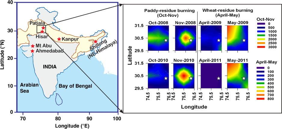
Fig. 1

2.2. Analytical methods

Aerosol samples were collected using a high-volume sampler (flow rate: 1.2 m³ minutes⁻¹) by filtering ambient air through the pre-combusted (at 350°C for ~6 h) tissuquartz filters (PALLFLEX™, 2500QAT-UP, 20 cm×25 cm). A total of 59 PM_2.5 samples were collected during paddy-residue burning emissions (October–November in 2008 and 2010), of which initial 33 samples were integrated for ~24 h each (in the first-campaign in 2008) and the remaining 26 samples for 8–10 h each (daytime in the second-campaign in 2010), to collect the adequate aerosol mass on tissuquartz filters. However, during wheat-residue burning emissions (April–May in 2009 and 2011), all samples (n=31) were collected during the daytime, integrating each sample for 8–10 h and so was the case during wintertime (n=51; December 8–March 9 and December 10–March 11). The meteorological conditions (temperature, relative humidity and wind) are nearly same from year-to-year during the paddy-residue burning emissions (October–November, 2008 and 2010), and so is the case during wheat-residue burning emissions (April–May, 2009 and 2011). The meteorological parameters (temperature, relative humidity and wind) during wintertime also do not exhibit inter-annual variability for the data set discussed in this study. The elemental carbon (EC) and organic carbon (OC) were measured on thermo-optical carbon analyser (Sunset Laboratory) using the NIOSH (National Institute for Occupational Safety and Health) protocol (Birch and Cary, 1996), water-soluble organic carbon (WSOC) on total OC analyser (Shimadzu; TOC 5000 A), water-soluble potassium on ion-chromatograph (Dionex®) and particulate-bound polycyclic aromatic hydrocarbons (here after referred as PAHs and in Table 1) on gas chromatograph coupled with a mass spectrometer (GC-MS, Agilent: 7890A/5975C) (Rengarajan et al., 2007; Rajput et al., 2011a, 2011b, 2013; Ram et al., 2012).

3.1. Aerosol characteristics from post-harvest biomass burning emissions in the IGP

Post-harvest paddy-residue (with moisture content: 40–50%) is burnt in open fields (under ambient atmospheric conditions of 24–30°C temperature and 51–65% relative humidity), during October–November in the IGP (Gupta et al., 2004; Badarinath et al., 2006; Punia et al., 2008). The post-harvest wheat-residue (with moisture content: <5%) is burnt under ambient temperature ranging from 33 to 38°C at low relative humidity (34–41%), during April–May. The PM_2.5 mass concentration averages around 200 µg m⁻³ during the paddy-residue burning emission (Table 1; Fig. 2) and ~50 µg m⁻³ during the wheat-residue burning emission. The average contributions of OC, EC and nss-K⁺ to PM_2.5 from paddy-residue burning emission are 33, 3.5 and 2.4%, respectively (Fig. 2). From wheat-residue burning emission, the average contributions of OC, EC and nss-K⁺ to PM_2.5 are 26, 7 and 2.4%, respectively.

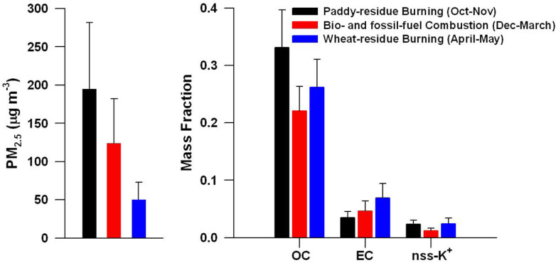
Fig. 2

The ΣPAHs (sum of 16 PAHs: 2- to 6-ring, reference is made to Table 1) average concentration from paddy-residue burning is 27.1 ng m⁻³ and from wheat-residue burning emission is 4.1 ng m⁻³. The contribution of 4- to 6-ring PAHs (Σ_{(4- to 6-)}PAHs) to the total PAHs (ΣPAHs) is 95±2% for the two biomass burning emission sources. Further differences in the two biomass burning emission sources are assessed by the relative distribution of ring-wise PAHs with respect to the 6-ring PAHs. The 4-/6-ring and 5-/6-ring distributions also exhibit significant differences between the two biomass sources: relatively high ratios are recorded for the paddy-residue burning emission. The ΣPAHs/OC ratio of 0.4 mg g⁻¹ from paddy-residue burning is relatively high (Table 1) than that from the wheat-residue burning emission (0.30 mg g⁻¹). Furthermore, the ΣPAHs/EC ratio of 4.3 mg g⁻¹ from paddy-residue burning is also higher (Table 1) than that from the wheat-residue burning emission (1.30 mg g⁻¹). The combustion of moist paddy-residue (with moisture content: 40–50%) during open biomass burning in October–November is responsible for higher contribution of OC to PM_2.5 and high-molecular weight PAHs (4- to 6-rings) in OC. In contrast, under dry weather conditions, the emissions from wheat-residue burning (with moisture content<5%) gives higher contribution of EC in PM_2.5 as compared to that from paddy-residue burning emission (EC/PM_2.5: 3.5%).

Based on linear regression analyses (p<0.0001) among OC, EC, nss-K⁺ and WSOC, the characteristic ratios of OC/EC, nss-K⁺/OC and WSOC/OC are constrained for the emissions from agricultural-residue burning (Table 1, Fig. 3). The OC/EC ratio of 10.6 for paddy-residue burning emission is significantly higher than that for the wheat-residue burning emission (3.0; Fig. 3a). The nss-K⁺/OC ratio of 0.06 for the paddy-residue burning emission is also different, lower by a factor of 2 than that from the wheat-residue burning emission (0.14; Fig. 3b). This is attributable to the high abundance of OC from paddy-residue burning emission. Furthermore, a major fraction of OC is found to be soluble in water from both the biomass burning emissions: the WSOC/OC ratio of 0.52 for paddy-residue is lower than that for the wheat-residue burning emission (0.60; Fig. 3c). In this context, an earlier study reports that the WSOC can have primary production from biomass burning emission as well as secondary formation pathway via photochemical reactions in the atmosphere (Mayol-Bracero et al., 2002). It is important to state here that a recent study from the Amazonian forest has suggested the significance of biogenic potassium to serving as a seed for SOA formation (Pöhlker et al., 2012). Thus, the SOA production can be favoured by their condensation onto K⁺ particles following the photochemical reactions of volatile organic compound (VOC) with atmospheric oxidants. In our context, it is likely possible that the biomass burning derived potassium could also serve as a seed for the SOA production. Relatively high abundances of nss-K⁺ and OC in PM_2.5 from paddy-residue burning emission would facilitate higher contribution of secondary organic carbon (SOC) than that from the wheat-residue burning (Fig. 3b; Table 1). Furthermore, during wintertime (December–March) the OC with EC and OC with nss-K⁺ suggests for the dominant impact from biomass burning emission in the IGP [OC/EC: 4.2; nss-K⁺/OC: 0.0.06]. The WSOC/OC ratio (0.62) in winter looks also similar to that observed from two distinct post-harvest biomass burning emissions (of paddy- and wheat-residue).

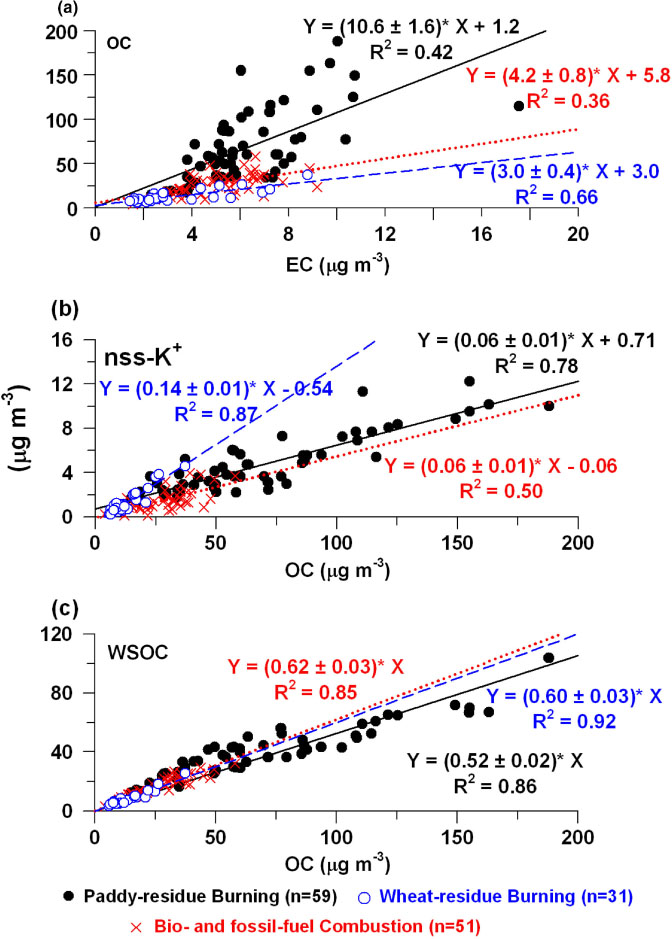
Fig. 3

PAH isomer ratios for the fossil-fuel combustion, forest fires and bio-fuels burning emission are available in the literature (Kirton et al., 1991; Khalili et al., 1995; Masclet et al., 1995; Schauer et al., 2001; Sheesley et al., 2003; Khillare et al., 2005a, 2005b). However, the information on PAH isomer ratios from the two potential sources of carbonaceous aerosols in the IGP, paddy- and wheat-residue burning (under ambient atmospheric conditions) is rather lacking in the literature (Rajput et al., 2011b). In this context, the present study serves to provide several PAH isomer ratios along with the major composition of carbonaceous species (EC, OC and WSOC) and nss-K⁺ in PM_2.5 from paddy- and wheat-residue burning emission for statistically significant number of data set (Table 1). Employing the PAH isomers, ANTH/(ANTH+PHEN) and IcdP/(IcdP+BghiP) against FLA/(FLA+PYR) in the cross plots, we document a characteristic information for the post-harvest agricultural-waste burning emissions from paddy- and wheat-residues (Fig. 4a and b; Table 1), distinctly different from the fossil-fuel combustion sources. The chemical characteristics of carbonaceous aerosols from biomass burning and fossil-fuel combustion sources in the IGP (from Patiala) during wintertime are summarised in Table 1 (for n=51).

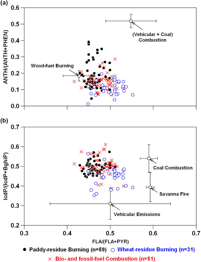
Fig. 4

3.2. OC/EC ratio during wintertime (December–March) from different geographical locations in India

Earlier studies conducted in the IGP have reported on the concentrations of OC and EC in total suspended particulate matter (TSP; Table 2) during the wintertime (December–March) (Rengarajan et al., 2007; Ram and Sarin, 2010). The spatial variability in average concentration of TSP was reported to be ~100–400 during the wintertime in the IGP. The average mass fractions of OC and EC are nearly identical varying from ~16–18 and 2–4%, respectively, at study locations (Table 2). Based on the aerosol composition analysis from December 2008 to March 2009 and December 2010 to March 2011 at Patiala in the IGP (this study), we find PM_2.5 concentrations varying from 19 to 244 (124±58) µg m⁻³ (Table and 2), quite similar to TSP from other locations in the IGP. The mass fractions of OC (22±4%) and EC (4.6±1.8%) in PM_2.5 at Patiala are also quite similar to that in TSP over other locations (Hisar, Kanpur and Allahabad) during the wintertime. Thus, contribution of fine-mode aerosols (aerodynamic diameter ≤2.5 µm) to TSP is dominant during the wintertime. The major source of particulate matter during the wintertime in the IGP is attributed to emissions from bio-fuel burning and fossil-fuel combustion sources (Rengarajan et al., 2007; Ram and Sarin, 2010; Rajput et al., 2011b).

Furthermore, downwind transport of pollutants from IGP along the foot-hills of NE-Himalaya, during the wintertime, has been documented by a recent study from NE-Himalaya [Barapani: 25.7°N, 91.9°E; 1064 m amsl; n=51, January–March 2009 and 2010], wherein PM_2.5 concentration varies from 39 to 348 (Av: 97±50) µg m⁻³: of which OC and EC contributes 36±8 and 6±3%, respectively (Rajput et al., 2013). The OC/EC ratio ~7.0 from the foot-hills of NE-Himalaya is similar to that observed from several locations in the IGP. In contrast, over northern Bay of Bengal (N-BoB: ~10–20°N latitude; n=31) the PM_2.5 concentration in the marine atmospheric boundary layer (MABL) varies from 13.2 to 76.7 (38±20) µg m⁻³; with contributions from OC and EC as 16 and 5%, respectively (Srinivas et al., 2011). The PM_2.5 concentration over the southern BoB (S-BoB: ~2–10°N latitude) varies from 2.0 to 35.3 (22.3±9.9) µg m⁻³; with contributions from OC and EC as 12 and 5%, respectively. Thus, OC mass fraction decreases, whereas EC contribution remains constant as a function of distance from the source region (with north-south gradient over open ocean). This is attributable to the preferential removal of OC (residing in coarse fraction) compared to EC (in fine fraction) in the MABL over the BoB. A systematic decrease in OC/EC ratio has been also observed over the Pacific in the outflow from East Asia (Lim et al., 2003). They attributed the decrease in OC/EC ratio to relatively longer atmospheric life-time of EC than OC in the MABL.

In order to assess the spatial distribution of carbonaceous aerosol in terms of OC/EC ratio from different geographical locations over India, aerosol sampling during wintertime from two additional sites, at Ahmedabad [23.03°N, 72.65°E; 49 m amsl; n=16, 1 December 2009–28 January 2010] and Mt Abu [24.6°N, 72.7°E; 1680 m amsl; n=15, 12 February–17 March 2010] in semi-arid region of western India, has been conducted in this study. The PM_2.5 concentration varied from 32 to 161 (Av±sd: 85±37) µg m⁻³, of which 33±6% is OC and 6±1% is EC at Ahmedabad. The PM_2.5 concentration varied from 10 to 38 (22±9) µg m⁻³, of which 10±6% is OC and 3.3±1.6% is EC at Mt Abu. It is relevant to state that during wintertime, prevailing NE-winds favour the long-range transport of pollutants from the IGP to western India. Thus, aerosols over Ahmedabad represent regional characteristics as well as components from long-range transport. However, the other site in western India at Mt Abu (1680 m amsl) is by-and-large impacted by the long-range transport.

The OC/EC average ratio as high as ~6–10 in the upwind locations in the IGP (Table 2) is attributable to the dominance of biomass burning emission sources and photochemical reactions (Rengarajan et al., 2007; Ram and Sarin, 2010; Rajput et al., 2011a). A similar OC/EC ratio of ~6 from Manora Peak and ~10 in aerosols from the southern slope of higher Himalaya (National Climate Observatory-Pyramid: NCO-P sampling station) have been also attributed earlier to the dominance of biomass burning emissions and/or contributions from SOA (Decesari et al., 2010; Ram et al., 2010). Furthermore, a similar OC/EC ratio from a semi-arid location at Ahmedabad (~6) is observed during wintertime. In contrast, at other places in India (Mumbai and Chennai), the OC/EC ratio is ~2–3 (Venkataraman et al., 2002; Pavuluri et al., 2011). However, the OC/EC ratio in winter over the BoB has been reported to be >2 (Srinivas et al., 2011). Thus, we integrate the present-day wintertime (December–March) scenario on significant variability in the chemical characteristics of carbonaceous aerosols in terms of the OC/EC ratio from the IGP and those over different environmental regions in and around the country.

3.3. Emission budget of carbonaceous species from paddy- and wheat-residue burning in the IGP

The emission of carbonaceous species (EC, OC and ΣPAHs) from the paddy- and wheat-residue burning in the IGP is estimated using the following equation:

Here, ‘EF’ is abbreviated for emission factor; ‘FL’ for fuel load over the agricultural fields and ‘AB’ for annual area burnt in the IGP (Table 3). A factor of 10⁻⁹ is multiplied to convert gram-emissions into Giga-grams (Gg).

In this study, the EF for carbonaceous species (EC, OC and ΣPAHs) from post-harvest paddy- and wheat-residue burning is suitably adopted from recent studies (Hays et al., 2005; Kanokkanjana et al., 2011). We have taken into consideration the differences in the OC/PM_2.5 and EC/PM_2.5 ratios for the biomass burning under ambient atmospheric conditions and those based on chamber experiments in order to assess the emission factors (Hays et al., 2005; Kanokkanjana et al., 2011). In case of paddy-residue burning emissions, the average mass fraction of (OC+EC)/PM_2.5 is 36.5±7.1% (this study). This mass fraction is in close agreement with that reported (38±2%) in a recent study (Kanokkanjana et al., 2011) for moist combustion of paddy-residue from irrigated fields. Therefore, we have adopted the EF of EC as 0.72±0.03 g/kg reported by (Kanokkanjana et al., 2011). The EF of OC is not assessed in their study on paddy-residue burning emissions, unlike our approach using the following equation:

And, the EF of ΣPAHs for paddy-residue burning is estimated from the mass fraction of PAH (ΣPAHs/OC), using the following equation:

For wheat-residue burning emissions, the mass fraction of OC (26±5%) in the IGP is quite similar to that reported from a chamber experiment (Hays et al., 2005). However, the contribution of EC (6.9±2.5%) in PM_2.5 from wheat-residue burning emission in the IGP is about 1.6 times lower as compared to 11% in the chamber (Hays et al., 2005). Therefore, we have used the same EF for OC and scaled down the EF of EC by a factor of 1.6 as reported by (Hays et al., 2005) for wheat-residue burning emission under ambient atmospheric conditions (Table 3). The EF of ΣPAHs for paddy-residue burning is estimated from eq. (3).

The value of fuel load (Table 3) for the paddy- and wheat-residues over the agricultural fields is adopted from a recent literature representing the agricultural-scenario for the states of Punjab in the IGP (Badarinath et al., 2006).

Based on the analysis of open fire-counts satellite data (Resolution: 1°×1°, latitude-longitude grid) from the MODIS (on-board Aqua/Terra; level 2) during 2008–2011, the fire active (agricultural-waste burning) area in the IGP (Fig. 1; including the states of Punjab, Haryana and western part of UP) is estimated to be 48400 sq. km (Justice et al., 2002). The fire-count data (Fig. 1) has been corrected for Cloud and Overpass. The ‘Cloud and Overpass corrected fire-pixel count’ represents the number of pixels corrected for multiple satellite overpass, missing observations and variable cloud cover (Justice et al., 2002). Since the region (upwind IGP) is fire active for a total of 4 months in a year: due to the practice of paddy-residue burning during October–November and wheat-residue burning during April–May. Therefore, it is considered logical to estimate the emission of aerosols in the IGP from the paddy- and wheat-residue burning only for 2 months each, and represented here as the total emission (Table 3).

3.4. A global scenario on biomass burning emissions

Recently the global emission budget of EC and OC has been revised (Bond et al., 2013). Accordingly, ~62 Tg/y of OC (primary) and ~14 Tg/y of EC are emitted from the biomass burning and fossil-fuel combustion sources over the globe. Between the two sources, emission from biomass burning is dominant: producing ~89% of the total OC and 60% of the total EC. Furthermore, among the biomass burning sources, the major source of OC (26 Tg/y) and EC (4.3 Tg/y) is the bio-fuel burning (Fig. 5). The emission from savanna fires produces ~17 Tg/y of OC and 2.2 Tg/y of EC. The forest fires produce ~17 Tg/y of OC and 1.5 Tg/y of EC. The agricultural-waste burning emissions are reported to produce 1154 Gg/y of OC and 280 Gg/y of EC on a global scale. In this context, the net emissions of OC and EC from agricultural-waste burning from the IGP (Northern India) are estimated as 505±68 and 59±2 Gg/y, respectively (Table 3). Using the EC-tracer method (Castro et al., 1999), it has been estimated that ~50% of the OC is primary during both the paddy- and wheat-residue burning emissions. Thus, the net emission of primary OC from agricultural-waste (paddy- and wheat-residue) burning is estimated as 252±34 Gg/y. As far as the emission budgets from the agricultural-waste burning on a global scale are concerned, ~22% of primary OC [252±34 Gg/y] and 21% of EC [59±2 Gg/y] are produced from the IGP (Northern India; Fig. 5). However, on a global biomass burning emission scale, as of present understanding, the contribution of primary OC and EC from the agricultural-waste burning emission is 2 and 3%, respectively (Bond et al., 2013).

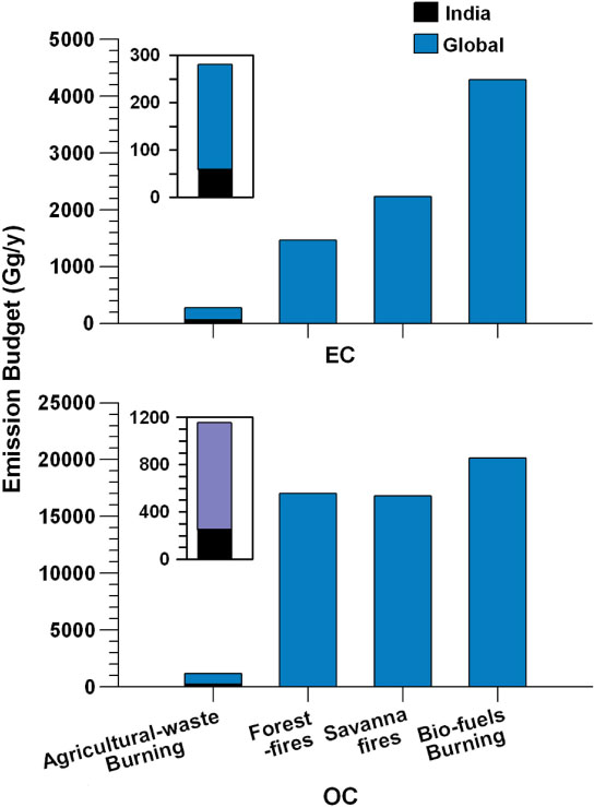
Fig. 5