
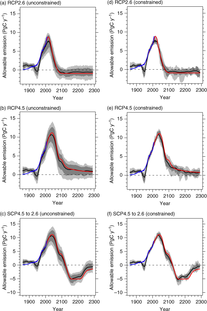
Fig. 1
Time series of allowable annual fossil fuel emissions for period 1850–2300.RCP2.6 (a), RCP4.5 (b) and SCP4.5 to 2.6 (c). The black curve is the ensemble mean, and the dark and light grey shades correspond to 68 (16–84 percentile) and 90 (5–95 percentile)% ranges respectively. The blue curve is the historical estimates of emissions (Carbon Dioxide Information Analysis Center: http://cdiac.ornl.gov/ftp/ndp030/global.1751_2009.ems). The red curves are harmonised RCP emissions (derived from MAGICC, documented in Meinshausen et al., 2011a). (d)–(f) are same as (a)–(c) but now for our constrained set of simulations using the eight observed datasets in Table 2.
Table 1
Parameters perturbed in this study and the ranges considered
[i] Parameters perturbed and where the symbols are: * and **: depth- and biome-dependent. †initially in a uniform distribution, and then weighted with a beta function (Appendix A1). ††Weighted with combination of two Gaussian functions (Appendix A2).
[ii] [a]: Gent and McWilliams (1990).
[iii] [b]: Tachiiri et al. (2010).
[iv] [c]: Oort (1983).
Table 2
Observation data used for constraint of simulations
[ii] *Effective ensemble size (EES) calculated as Σ(weights)/Σ(weights)2. EES becomes large when the weights are equally distributed across many members, and small when weights are concentrated on small numbers of members. **0.18 for 90% confidence level. ***Compared with the model's allowable emission for these periods. †These SD values are used to calculate the weight similar to CPI (Murphy et al., 2004). ††The values are SDs for 0–50/50–600/600–2000/2000–5500 m.
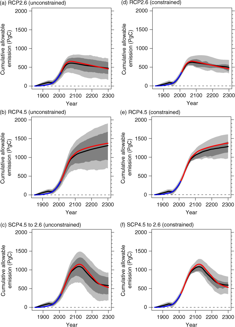
Fig. 2
Time series of cumulative allowable emissions for period 1850–2300.
RCP2.6 (a), RCP4.5 (b) and SCP4.5 to 2.6 (c). The black curve is the ensemble mean, and the dark and light grey shades correspond to 68 (16–84 percentile) and 90 (5–95 percentile)% ranges respectively. The blue curve is the historical estimates of emissions (Carbon Dioxide Information Analysis Center: http://cdiac.ornl.gov/ftp/ndp030/global.1751_2009.ems). The red curves are harmonised RCP emissions (derived from MAGICC, documented in Meinshausen et al., 2011a). (d)–(f) are same as (a)–(c) but now for our constrained set of simulations using the eight observed datasets in Table 2.
Table 3
Comparison of cumulative fossil fuel emission with CMIP5 models
Table 4
Allowable fossil-fuel emissions for 1990s and 2050s for RCP2.6
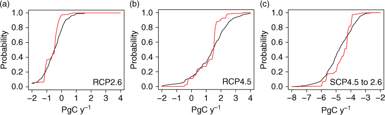
Fig. 3
The cumulative probability distribution for allowable emission thresholds when averaged over the period of years 2151–2200.
RCP2.6 (a), RCP4.5 (b) and SCP4.5 to 2.6 (c). The cumulative probability of these mean emissions being less than each threshold presented on the x-axis. Presented are the weighted probability for the unconstrained (black curve), and constrained ensembles using all variables in Table 2 (red curve).
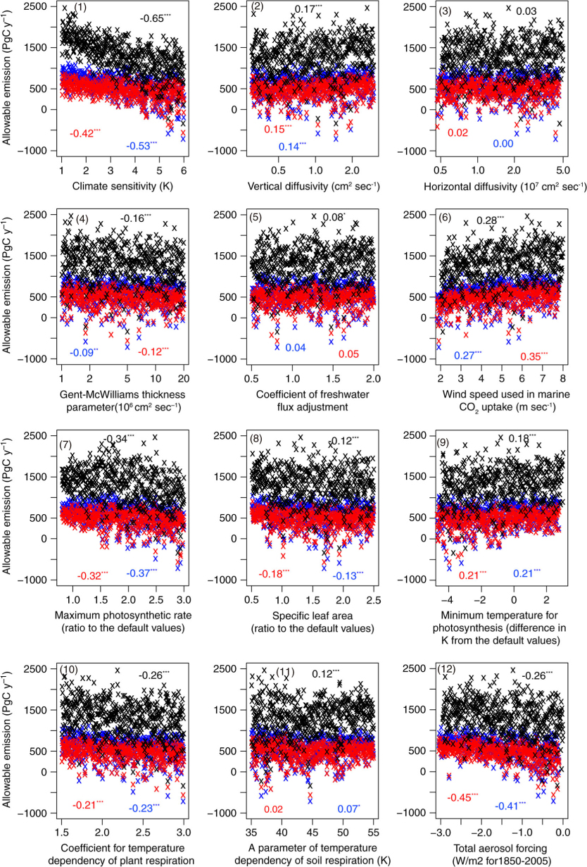
Fig. 4
Relationship between the cumulative allowable emission (1850–2300) and variation in different parameter values.
RCP2.6 (red), RCP4.5 (black) and SCP4.5 to 2.6 (blue). Panels (1)–(12) are in the same order as Table 1. Numbers in plot areas are coefficients of correlation to parameter values (*/**/*** mean statistically significant at 90/95/99% levels). Plotted are the 512 members.
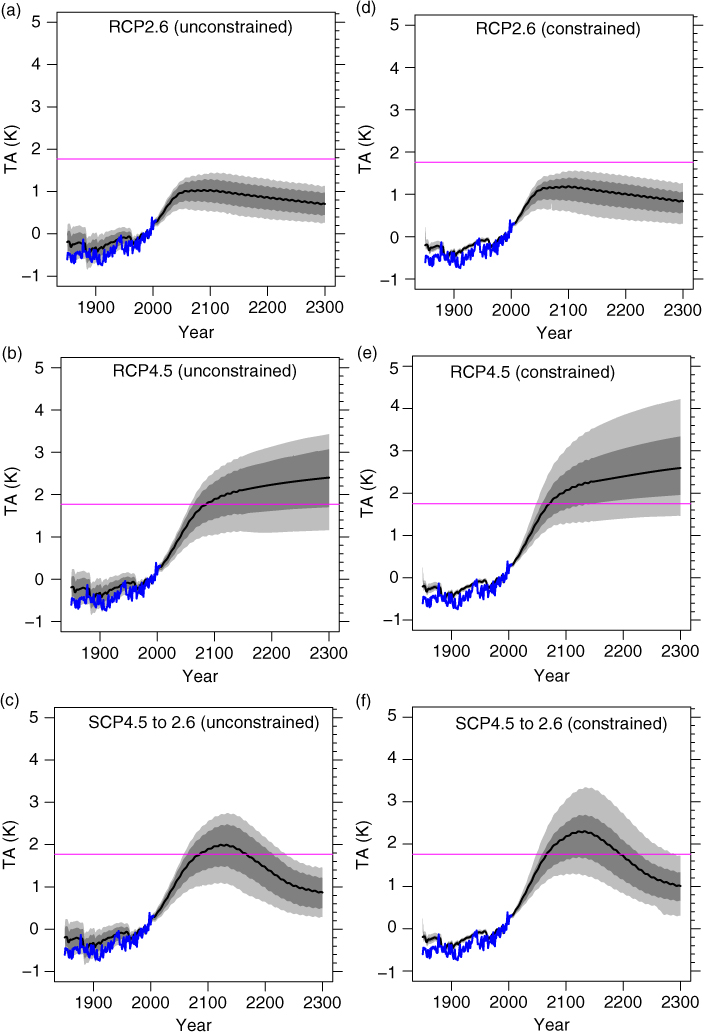
Fig. 5
Time series of global mean surface air temperature for period 1850–2300.
RCP2.6 (a), RCP4.5 (b) and SCP4.5 to 2.6 (c). The black curve is the ensemble mean, and the dark and light grey shades correspond to 68 (16–84 percentile) and 90 (5–95 percentile)% ranges respectively. The blue curve is the HadCRUT3 data (Brohan et al., 2006). Anomalies are from average of 1980–1999, and the horizontal magenta line is 2 K increase from the preindustrial (here average of 1850–1869). (d)–(f) are same as (a)–(c) but now for our constrained set of simulations using the eight observed datasets in Table 2.
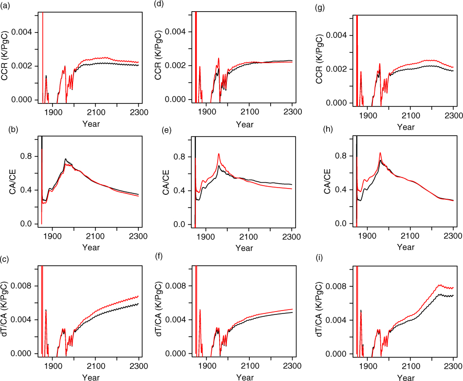
Fig. 6
Carbon Climate Response.
RCP2.6 (a–c), RCP4.5 (d–f) and SCP4.5 to 2.6 (g–i). The left (a, d, g), the central (b, e, h) and right (c, f, i) columns show Carbon Climate Response (ratio of temperature rise, dT, and cumulative emission (CE), ratio of CA (airborne carbon) and CE (i.e. airborne fraction) and dT/CA, respectively. Black and red lines are the unconstrained and the constrained ensemble average.
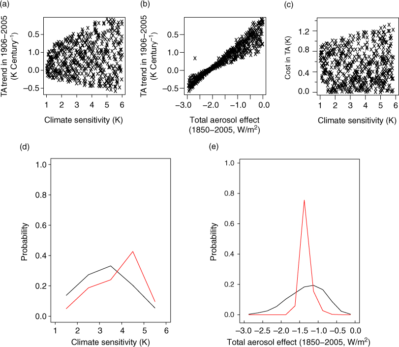
Fig. 7
The dependence of temperature trend (warming between years 1906 to 2005), plotted against (a) climate sensitivity, (b) uncertainty in aerosol forcing. Also plotted, (c) is the cost (errors defined as absolute value of the difference) in TA trend vs climate sensitivity. Plotted are all of the 512 members. (d) and (e) are prior and posterior of climate sensitivity and aerosol forcing, in which black: unconstrained, red: constrained. Plotted are probabilities for bins of 0.1 K (d) and 0.5 W/m2 (e) width.
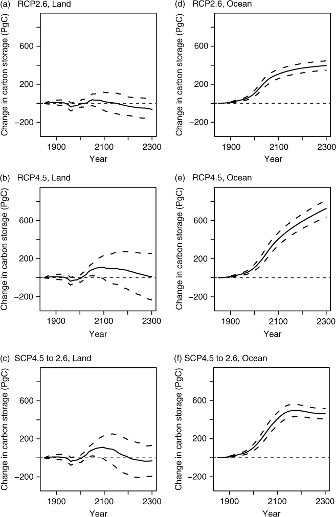
Fig. 8
Land and ocean carbon storage.
(a)–(c) are change in land carbon storage after constraint for RCP2.6, RCP4.5 and SCP4.5 to 2.6, respectively, and where a positive value implies a gain in carbon. The dark and light grey shades correspond to 68 (16–84 percentile) and 90 (5–95 percentile)% ranges respectively. (d)–(f) are change in ocean carbon storage for the scenarios.
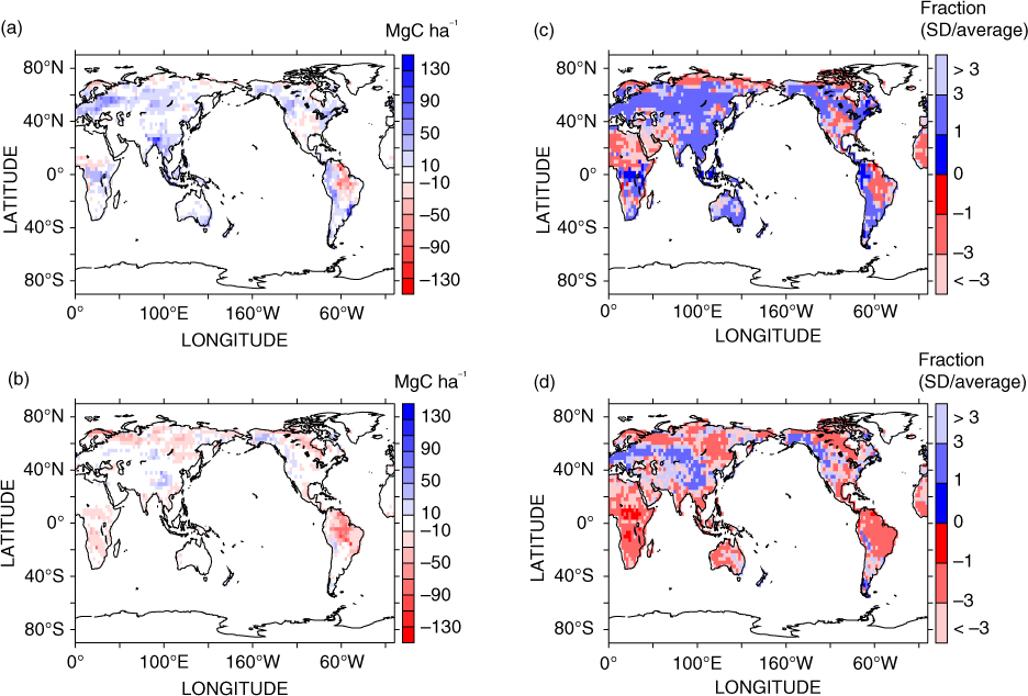
Fig. 9
Spatial distribution of the land carbon uptake.
Panel (a) is the weighted mean of land carbon uptake between 2010–2100 (i.e. year 2100 values minus year 2010 values), and (b) is land carbon uptake in 2100–2300. After constraint. Then panels (c) and (d) are relative uncertainty across the ensemble, calculated as SD/average in (a) and (b) respectively, presenting the extent of the consistency in the sign of change. When ∣SD/average∣ < 1, the sign of the change is considered be robust (note that the sign of ∣SD/average∣ simply presents that of average, as SD is always positive). Few grids are of robust signs for the change in 2010–2100, and even fewer grids are so in 2100–2300.
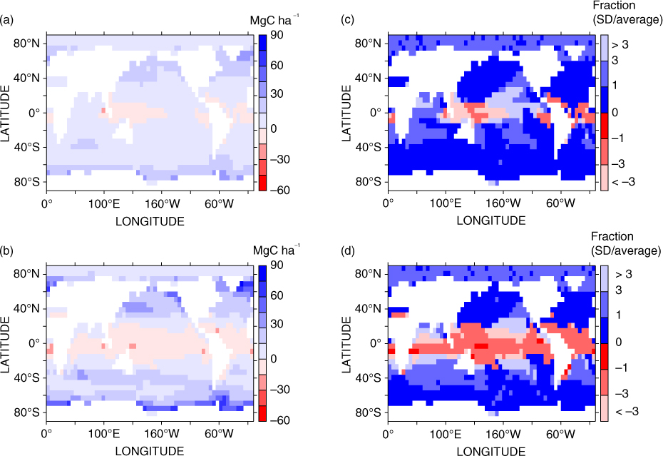
Fig. 10
Spatial distribution of the ocean carbon uptake (a): For 2010–2100, (b): 2100–2300, (c)(d): relative uncertainty (standard deviation/average). After constraint.
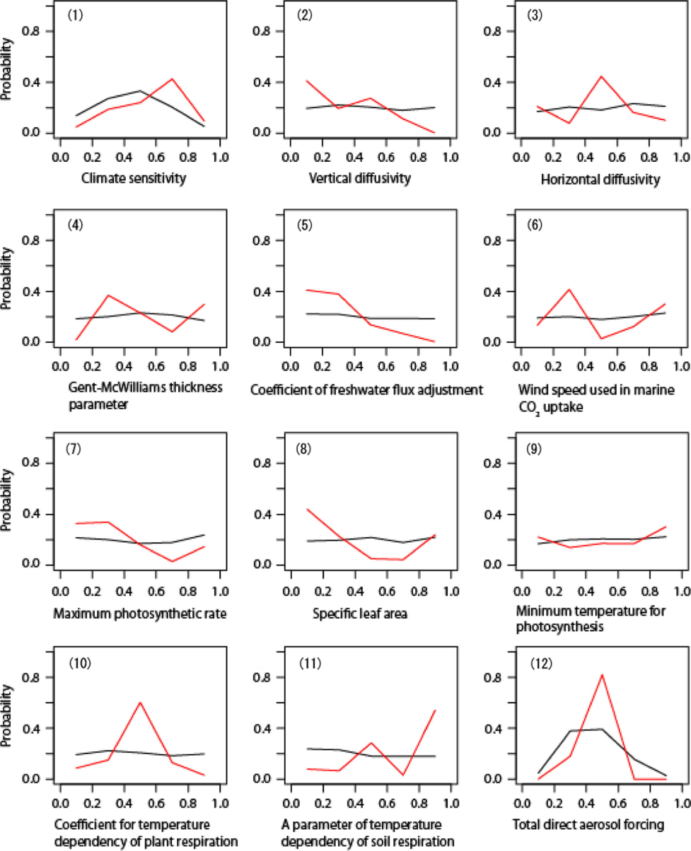
Fig. E1
Prior and posterior probability distribution of 12 parameters. Black: prior (unconstrained), red: posterior (after constrained by observation data). X-axis is normalised to the perturbation range (logarithmic scales for 2–4). Priors are flat for all parameters but climate sensitivity and aerosol for which non-flat distributions presented in Appendix A are used. Plotted are probabilities for bins of 0.2 (i.e. one fifth of the pertubed range) width.
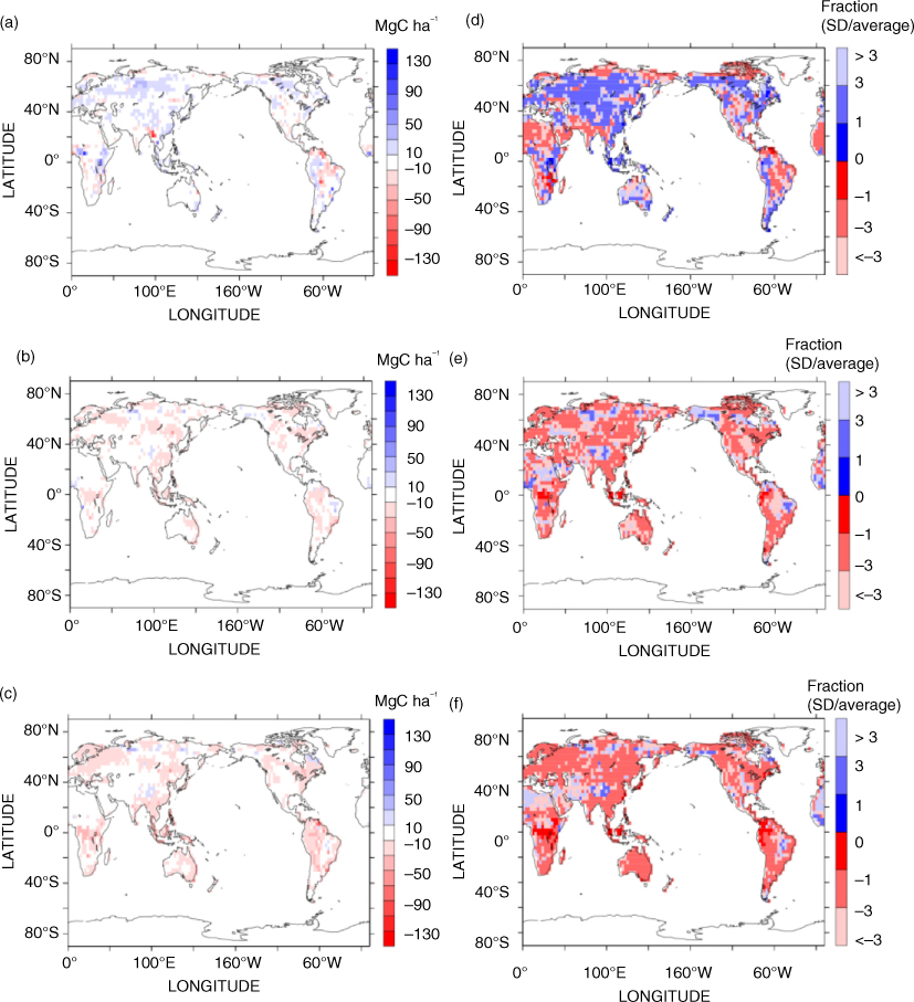
Fig. F1
Spatial distribution of the change in land carbon storage for RCP2.6 and SCP4.5 to 2.6. Panel (a) is the weighted mean of land carbon uptake between 2010 and 2100 (i.e. year 2100 values minus year 2010 values), and (b) is land carbon uptake in 2100–2300 for RCP2.6. (c) is land carbon uptake in 2100–2300 for SCP4.5 to 2.6. Then panels (d)–(f) are relative uncertainty across the ensemble, calculated as SD/average in (a)–(c) respectively. After constraint.
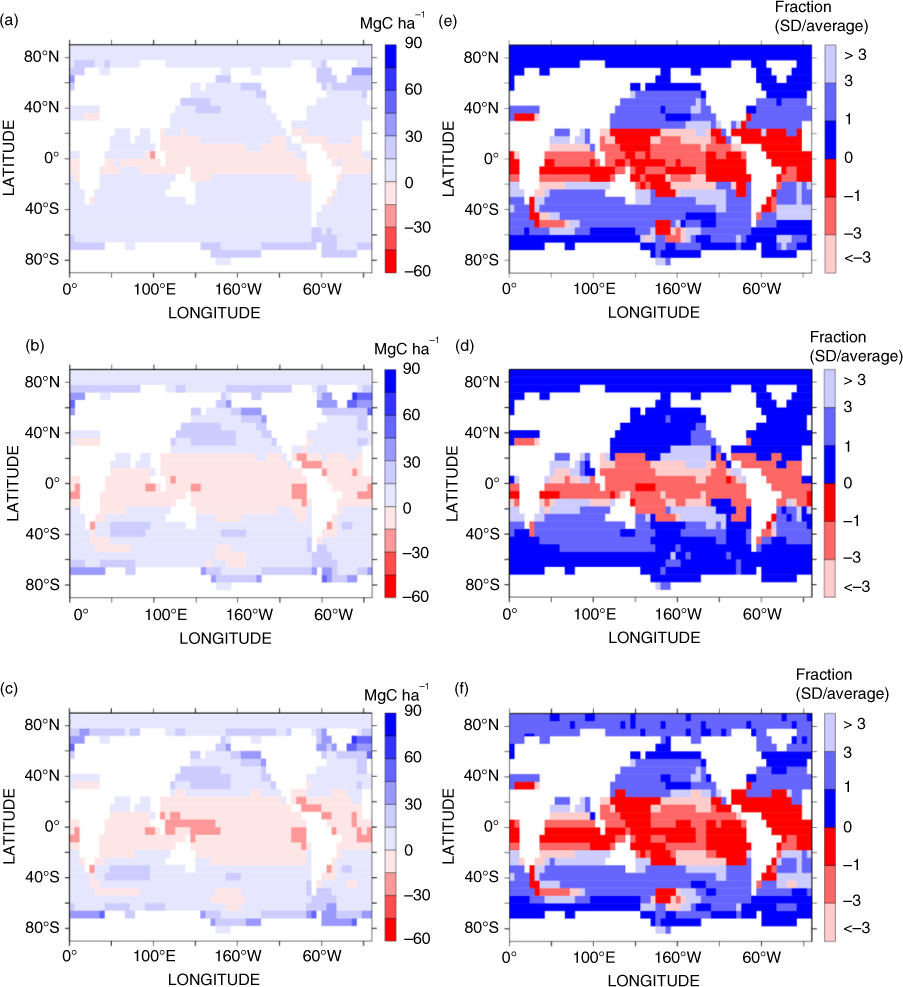
Fig. F2
Ocean carbon uptake (a) for 2010–2100, (b) 2100–2300 for RCP2.6, (c) 2100–2300 for SCP4.5 to 2.6, (d)–(f) relative uncertainty (standard deviation/average) for (a)–(c). After constraint.
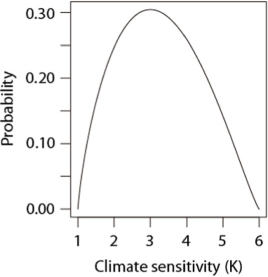
Fig. A1
The beta distribution with values B(1.8, 2.2), used to represent the asymmetric climate sensitivity's probability distribution.
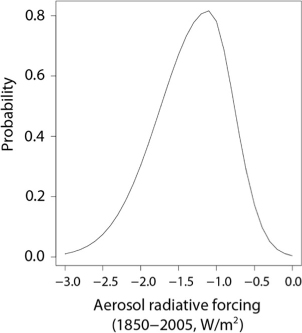
Fig. A2
The distribution of aerosol represented using a combination of two normal functions.
Table B1
. Feedback parameters compared to the C4MIP models
[i] Parameters presented (Friedlingstein et al., 2006), are linear transient climate sensitivity (α), sensitivity of land and ocean carbon storage to atmospheric CO2 concentration change (β) and to temperature change (γ). “l” and “o” are land and ocean. The ± one SD of 20 members (in a small ensemble) and also for C4MIP models are presented.
Table B2
. Original parameter perturbation ranges before the tuning for the C4MIP models
Table G1
. Result of the sensitivity tests for climate sensitivity with RCP4.5