
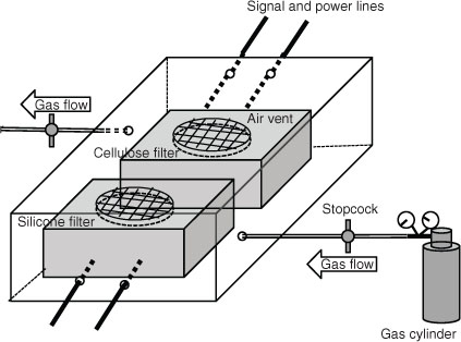
Fig. 1
Schematic of laboratory experiment.
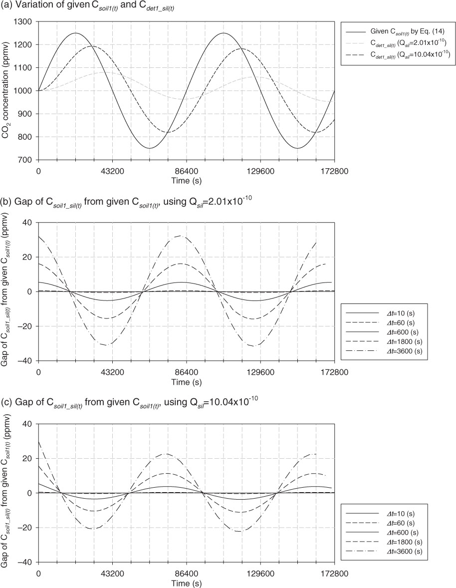
Fig. 2
(a) Time variations of given C soil(t) (black solid line) by eq. (14) and C det_sil(t) with Q sil=2.01×10⁻¹⁰ and 10.04×10⁻¹⁰ mol m m−2 s−1 kPa−1 (grey dashed line and black dashed line, respectively); (b) Time variation of the gap of C soil_sil(t) from given C soil(t), using Q sil=2.01×10⁻¹⁰ mol m m−2 s−1 kPa−1 and eq. (13). A negative value means that C soil_sil(t) is smaller than the given C soil(t). Five lines for five logging intervals (10 s, 1 min, 10 min, 30 min and 60 min) are shown; and (c) Time variation of the gap of C soil_sil(t) from given C soil(t), using Q sil=10.04×10⁻¹⁰ mol m m−2 s−1 kPa−1 and eq. (13). Lines are depicted as (b).
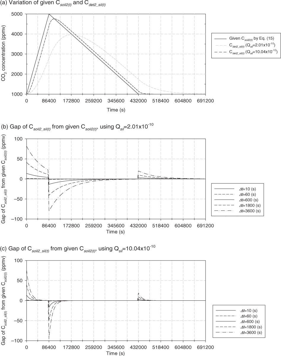
Fig. 3
(a) Time variations of given C soil(t) (black solid line) by eq. (15) and C det_sil(t) with Q sil=2.01×10⁻¹⁰ and 10.04×10⁻¹⁰ mol m m−2 s−1 kPa−1 (grey dashed line and black dashed line, respectively); (b) Time variation of the gap of C soil_sil(t) from given C soil(t), using Q sil=2.01×10⁻¹⁰ mol m m−2 s−1 kPa−1 and eq. (13); (c) Time variation of the gap of C soil_sil(t) from given C soil(t), using Q sil=10.04×10⁻¹⁰ mol m m−2 s−1 kPa−1 and eq. (13). Lines are depicted as Fig. 2.
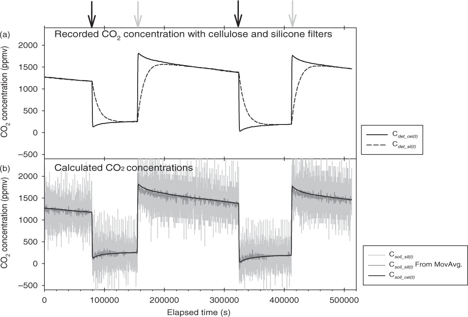
Fig. 4
(a) Time variation of C det_cel(t) (solid line) and C det_sil(t) (dashed line) responding to CO2 concentration in the container. Black and grey arrows respectively indicate the time to infuse the N2 and air-balanced CO2 standard (1930 ppmv) gases; and (b) time variation of C soil_sil(t) (grey line), C soil_sil(t) calculated from 60-data (10 min) moving averages of C det_sil(t) (dark grey line) and C soil_cel(t) (black line). These variations are calculated with Q sil=11.5×10⁻¹⁰ mol m m−2 s−1 kPa−1. Black solid lines do not denote the moving average of the grey solid line. C soil_sil(t) and C soil_cel(t) are calculated with eq. (13).
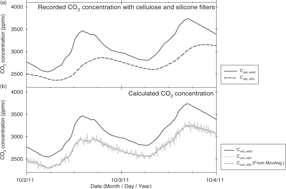
Fig. 5
Observed diurnal variations of CO2 concentration in the field experiment. (a) C det_cel(t) (solid line) and C det_sil(t) (dashed line); (b) C soil_cel(t) (black line), C soil_sil(t) (grey line) and C soil_sil(t) calculated from six-data (60 min) moving averages of C det_sil(t) (dark grey line). These variations are calculated with Q sil=11.5×10⁻¹⁰ mol m m−2 s−1 kPa−1. Black solid lines do not show the moving average of the grey solid line.
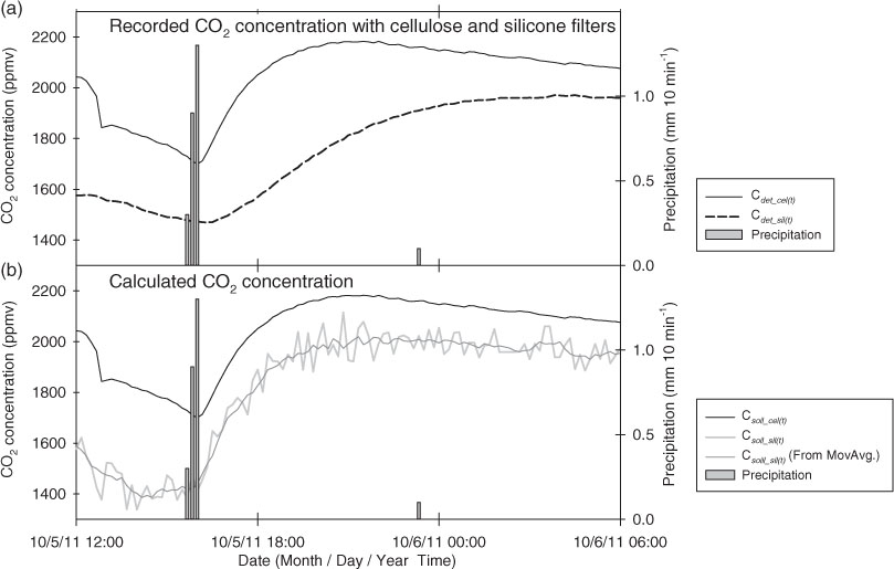
Fig. 6
Observed time variations of CO2 concentration after rainfall in the field experiment. (a) C det_cel(t) (solid line) and C det_sil(t) (dashed line); and (b) C soil_cel(t) (black line), C soil_sil(t) (grey line) and C soil_sil(t) calculated from 6-data (60 min) moving averages of C det_sil(t) (dark grey line). These variations are calculated with Q sil=11.5×10⁻¹⁰ mol m m−2 s−1 kPa−1. Black solid lines do not show the moving average of the grey solid line.