
1. Introduction
Installing a diffusion model CO2 sensor in the soil is one method to measure the gas CO2 concentration in the soil (e.g. Hirano et al., 2003; Tang et al., 2003; Chen et al., 2005; Liang et al., 2010; Pingintha et al., 2010). One important benefit of this method is that it can directly measure the time variation with high resolution. Moreover, it does not disturb the soil pores because of its artificial air flow once it is installed. Different from occasional manual observation, this measurement can be implemented irrespective of weather conditions. However, this method is usually inapplicable to a flooded field (e.g. farmland with snow melt, wetland with varying water levels).
Nevertheless, some studies have sampled soil gas from hydrophobic silicone tubes installed in the soil, and subsequently measured CO2 concentrations of the sampled gas in a laboratory (e.g. Holter, 1990; Syväsalo et al., 2004; Yanai et al., 2011). Using such a method, sampling can be done in waterlogged or temporary saturated fields, and spatial averages can be found using a certain length tube. DeSutter et al. (2006) reported another important feature: silicone is cheaper than other hydrophobic materials. Yanai and Tokida (2009) reported that the silicone tube permeability is higher than that of other hydrophobic materials, although the gas permeability of silicone is lower than that of widely used polytetrafluoroethylene (PTFE), which cannot be used under waterlogged conditions. However, this occasional measurement cannot evaluate time variation in high resolution.
Some studies have used silicone (or other hydrophobic material) tubes or tubes covered with silicone in the soil to analyse CO2 concentrations by circulating or flushing the air in the tube to the equipped analyser. This method can be operated automatically. However, this measurement system is bulky and needs several additional materials (e.g. gas cylinder, pump) (e.g. Flechard et al., 2007; Panikov et al., 2007).
Other reports have described studies that have used diffusive-type CO2 sensors covered with hydrophobic (e.g. silicone, Teflon) membrane (Jassal et al. 2004; Deppe et al. 2010), but the reports do not describe the inherent permeating time lag. To evaluate the time variation accurately, this lag must be considered.
This study examined the practical application of a silicon-covered sensor in field experiments, especially how accurately the variation of soil gas CO2 concentration can be estimated from the series of data obtained with a silicone-covered sensor.
2. Measurements
Two 98×64×35 mm (W×D×H) BEC-CO2SA sensor boxes (Baron Electric Co. Inc., Tokyo, Japan) were used. An infrared gas sensor module for CO2 sensing (CO2 Engine K30; SenseAir, Delsbo, Sweden) is installed in this CO2 sensor box. This module uses a non-dispersive infrared absorption (NDIR) method for CO2 sensing. Electricity consumption is 0.48 W with a 12-V current. The sensing volume is 8.0×10⁻⁵ m3. The measurement range is 0–5000 ppm with 1–5 V output and accuracy of ±30 ppmv±5% of measured values. The response time to 63% of a signal is 20 s. The output depends only slightly on the ambient temperature. Initially, a 4-cm diameter air vent was sealed with a cellulose filter using a rubber O-ring from the inside. The vent is protected from the outside by an aluminium mesh. The thickness and gas permeability coefficient for CO2 (Q, mol m m−2 s−1 kPa−1) of the cellulose filter, for which data are provided from the manufacturer, are 1.60×10⁻⁴ m and 1.03×10⁻³, respectively (Q cel, mol m m−2 s−1 kPa−1). These values reflect that the cellulose filter prevents gas permeation only slightly. A silicone filter was installed on one of the two sensors instead of a cellulose filter. The silicone filter thickness is 5.0×10⁻⁴ m. The information of Q of the silicone filter (Q sil, mol m m−2 s−1 kPa−1) is not available from the manufacturer.
For laboratory experiments, two CO2 sensor boxes with cellulose and silicone filter were placed in a 1950 ml plastic container (Fig. 1). Cables for the signal and power supply from the sensor boxes exited through the drilled hole of the plastic container. Reference gases were injected through the urethane tube (4-mm inner diameter) to the plastic container. The air exits through the urethane tube attached at the other side. The gas was closed using a stopcock attached to the tubes. N2 and air-balanced CO2 standard (1930 ppmv) gases were injected by turns. Gaps were sealed with epoxy resin adhesive to prevent gas leaks. The sensor output was recorded every 10 s using a voltage recorder (VR-71; T&D, Nagano, Japan). Its resolution was 5 mV or more. To remove periodical electric noise every minute, a moving average of six data was used. Ambient air temperature was recorded every minute using a thermo-recorder (TR-72S; T&D, Nagano, Japan). The temperature was assumed to vary linearly among recorded data.
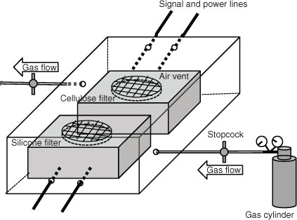
Fig. 1
Schematic of laboratory experiment.
As for field experiments, the two sensor boxes were installed with cellulose and silicone filter at 10 cm depth of bare soil. The sensors were placed with the air vent side downward. The sensor output was recorded every 10 min by averaging the 10 outputs at every minute using a data logger (CR1000; Campbell Scientific Inc., Logan, UT, USA) with a resolution of 1333 µV. Soil temperature at 10 cm depth was measured using a copper–constantan thermocouple. Precipitation was measured using a tipping-bucket rain gauge (Model 52202; R. M. Young Co., Traverse City, MI, USA). These were recorded every 10 min. Soil temperature was recorded by averaging the 60 outputs every 10 s. Data from 2–3 October 2011 and 5–6 October 2011 were used.
3. Calculation
I assumed that no driving force causes significant advective flow through the membrane, and that gas permeation velocity v (mol s−1) is expressed as the following widely used equation (e.g. Brandrup and Immergut, 1989):
where A (m2) is the polymeric membrane filter area, δ (m) is the membrane thickness, and Δp (kPa) is the difference of membrane partial pressure (inside vs. outside). In this study, CO2 concentration was assumed to be uniform inside the sensor. At time t (s), assuming atmospheric pressure in the sensor P (t) (kPa) is equivalent to that in the soil, v (t) is expressed aswhere C soil(t) (ppmv) and C room(t) (ppmv) denote the CO2 concentrations in the soil and the sensing room, respectively. At this time, assuming that CO2 gas is always distributed uniformly in the sensing room, the number of moles of total gases N total(t) (mol) in the sensing room of the sensor is expressed as follows:
where R represents the gas constant 8.31×10⁻³ (kPa m3 mol−1 K−1), T (t) (K) represents temperature, and V (m3) represents the sensing volume inside the sensor. Therefore, the rate of increase in the CO2 concentration in the sensing room C′ room(t) (ppmv s−1) is expressed by the following equation:C′ room(t) can be assumed to be constant during the micro time period (from t to t+Δt). Probable errors depending on the scale of Δt are shown in Sections 4.1 and 4.2. In this case, the increase in CO2 concentration in the sensing room from at t to at t+Δt can be expressed as C′ room(t)Δt. Therefore, at time Δt (s) after time t, the CO2 concentration in the sensing room is as follows:
Transforming this equation, C soil(t) is the value shown below.To express the response character of the detector, which finally outputs the signal of CO2 concentration, there are some conceivable response functions (e.g. Robert, 1993). I applied the simple time response function in the first-order system because of the limited technical information of the sensor. After the CO2 concentration in the room is replaced with C room at t=0 from the state that the sensor stably outputs the constant CO2 concentration in the room (C det(0)), C det(t) would be expressed as follows:
where C det(t) is the detected CO2 concentration (ppmv), C room is a constant, and a is a coefficient. The CO2 sensor specifications imply the following equation:At this time,The rate of increase in the detected CO2 concentration C′ det(t) (ppmv s−1) is calculated from the time derivative of both sides in eq. (7). Furthermore, constant C room is replaced with C room(t) because C room(t) is assumed to be constant during the micro time period Δt for each calculation step.Transforming this equation, C room(t) is expressed as shown as follows:
When a cellulose filter is used, C soil=C room can be assumed. This is because the cellulose filter prevents gas permeation only slightly as described in Section 2. Therefore,Combining eqs. (6) and (11), C soil(t) is expressed as follows:
The precision with which C soil(t) was estimated was deduced theoretically with eq. (13) from recorded data of C det(t), depending on the length of the logging interval (i.e. Δt). According to a report by Lebovits (1966), Q sil was 2.01×10⁻¹⁰–10.04×10⁻¹⁰ mol m m−2 s−1 kPa−1. These minimum and maximum values were used in this study for theoretical calculations.
Hereinafter, the outputs of the cellulose-covered and silicone-covered sensor are denoted as C det_cel(t) and C det_sil(t), respectively. C soil(t) is calculated from C det_cel(t) or C det_sil(t) using eq. (13). These calculated C soil(t) are represented as C soil_cel(t) and C soil_sil(t), respectively.
4. Results
4.1. Theoretical uncertainty of the calculated Csoil(t) in diurnal variation
The diurnal variation of soil CO2 concentration was assumed depending on the soil temperature, as expressed by the following equations:
In these equations, C room1(0) and C det1(0) denote the initial recorded C room1(t) and C det1(t), respectively. Subscript ‘1’ is used in this exercise (e.g. C soil1(t), C room1(t), C det1(t) and T 1(t)). C det_sil(t) was calculated as follows. First, this author set C room(0)=C soil(0) and C det(0)=C soil(0) and then set Δt=1 (s) and calculated C room(t) and C det(t) step-by-step every second. Second, this author calculated C room(t+Δt) using the data C soil(t) and C room(t) with eq. (5). Finally, this author calculated C det(t+2Δt) using the data C room(t+Δt) and C det(t+Δt) with eq. (11), replacing t with t+Δt. In this exercise, Δt=1 is assumed to be a sufficiently short interval for calculation because a negligible gap (less than 1.1×10⁻⁷%) exists between calculated C det1(t) with Δt=1 and that with Δt=0.2 (data not shown), and this result implies that calculated C det1(t) with infinitesimal Δt has insignificant difference with calculated C det1(t) with Δt=1. Such diurnal variation described by C soil1(t), was described in earlier studies (e.g. Tang et al., 2003; Chen et al., 2005; Panikov et al., 2007; DeSutter et al., 2008). For this study, 10 s, 1 min, 10 min, 30 min and 1 hr were set as logging intervals.The variation of given C soil1(t) by eq. (14) and C det1_sil(t) is presented in Fig. 2a. The second positive peak of C det_sil(t) lags that of C soil1(t) 10 392–18 297 s (about 3–5 h). The value depends on Q sil. The gap separating C soil1(t) and C det1_sil(t) is 172.5–250.7 ppmv at most, whereas the gap separating C soil1(t) and C det1_cel(t) is 0.367 ppmv at most. Figure 2b and c shows the gap of C soil_sil(t) at each logging interval from C soil1(t). A negative value signifies that C soil_sil(t) is less than C soil1(t). Apart from the gap at the beginning, the gap is 5.4 ppmv, which is equivalent to 1.08% of the amplitude of C soil1(t), at Δt=600.
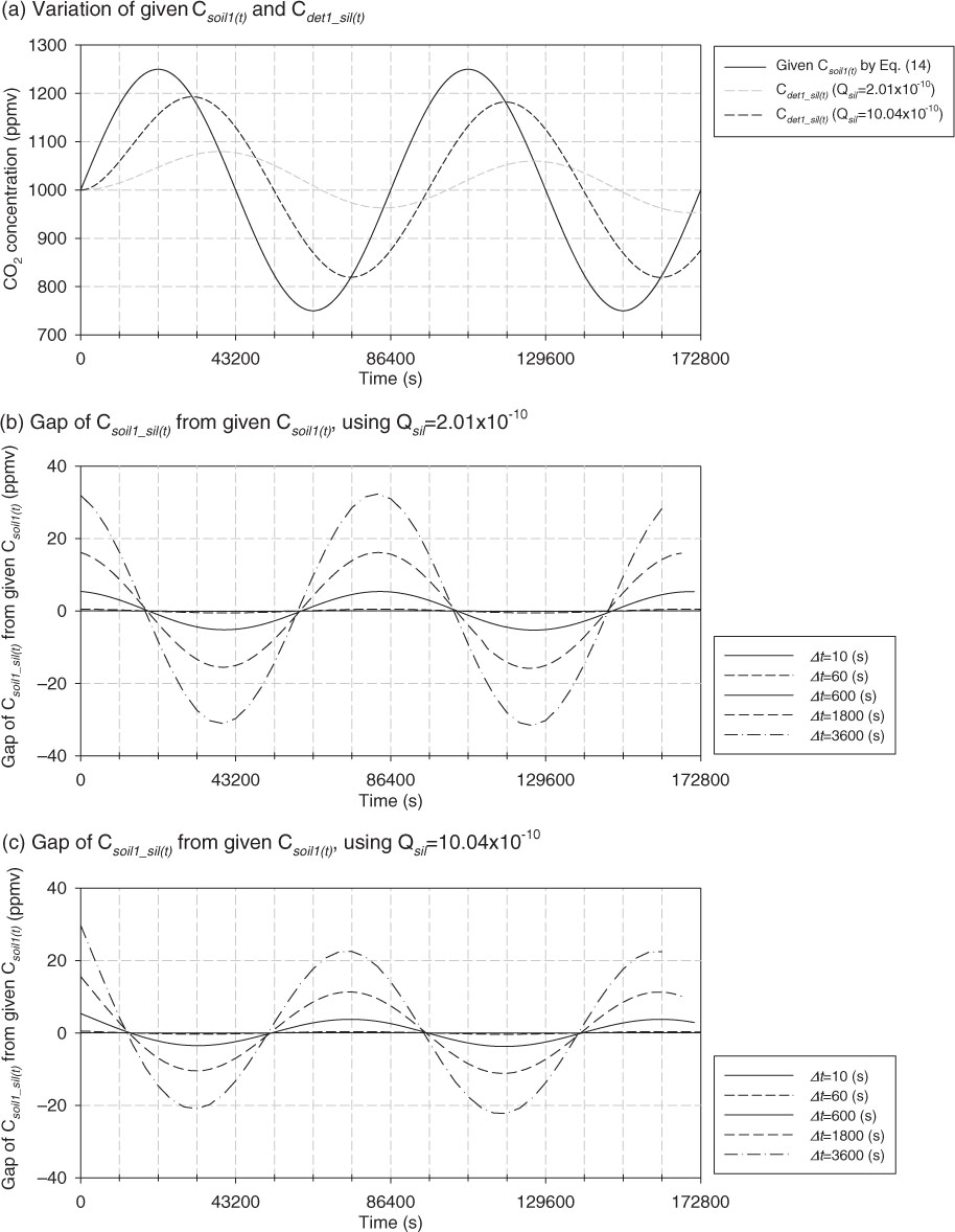
Fig. 2
(a) Time variations of given C soil(t) (black solid line) by eq. (14) and C det_sil(t) with Q sil=2.01×10⁻¹⁰ and 10.04×10⁻¹⁰ mol m m−2 s−1 kPa−1 (grey dashed line and black dashed line, respectively); (b) Time variation of the gap of C soil_sil(t) from given C soil(t), using Q sil=2.01×10⁻¹⁰ mol m m−2 s−1 kPa−1 and eq. (13). A negative value means that C soil_sil(t) is smaller than the given C soil(t). Five lines for five logging intervals (10 s, 1 min, 10 min, 30 min and 60 min) are shown; and (c) Time variation of the gap of C soil_sil(t) from given C soil(t), using Q sil=10.04×10⁻¹⁰ mol m m−2 s−1 kPa−1 and eq. (13). Lines are depicted as (b).
4.2. Theoretical uncertainty of the calculated Csoil(t) during a rainfall event
The sudden increase and decrease in soil CO2 concentration caused by rainfall events are assumed to be expressed as the following equations:
In these equations, C room2(0) and C det2(0) denote the initial recorded C room2(t) and C det2(t), respectively. Subscript ‘2’ is used in this exercise as in Section 4.1. C det2(t) was calculated as in Section 4.1. In this exercise, I also assumed that Δt=1 is a sufficiently short interval for calculating C det2(t). The gap separating calculated C det2(t) with Δt=1 and that with Δt=0.2 is also negligible (5.8×10⁻⁴%, data not shown).
Such variation was shown in earlier studies as well (e.g. Chen et al., 2005; DeSutter et al., 2008). Five logging intervals were set as examining diurnal variation. The variation of given C soil2(t) by eq. (15) and C det2_sil(t) is depicted in Fig. 3a. The positive peak of C det2_sil(t) delays from those of C soil2_(t) 20 952–89 175 s (about 6–25 h). The gap of C det2_sil(t) from C soil2(t) ranges from –2213 to 738 ppmv with Q sil=2.01×10⁻¹⁰ mol m m−2 s−1 kPa−1, and from −602 to 151 ppmv with Q sil=10.04×10⁻¹⁰ mol m m−2 s−1 kPa−1, whereas the gap separating C soil2(t) and C det2_cel(t) is 0.93 ppmv at most. Figure 3b and c shows the gap of C soil2_sil(t) at each logging interval from C soil2(t). The gap is 17.1 ppmv at most at Δt=600, which is equivalent to a 0.43% increase from initial C soil2(t) (1000 ppmv) to the peak (5000 ppmv). The gap becomes large when the change in increasing (or decreasing) rate of C soil2(t) becomes large, especially around the positive peak.
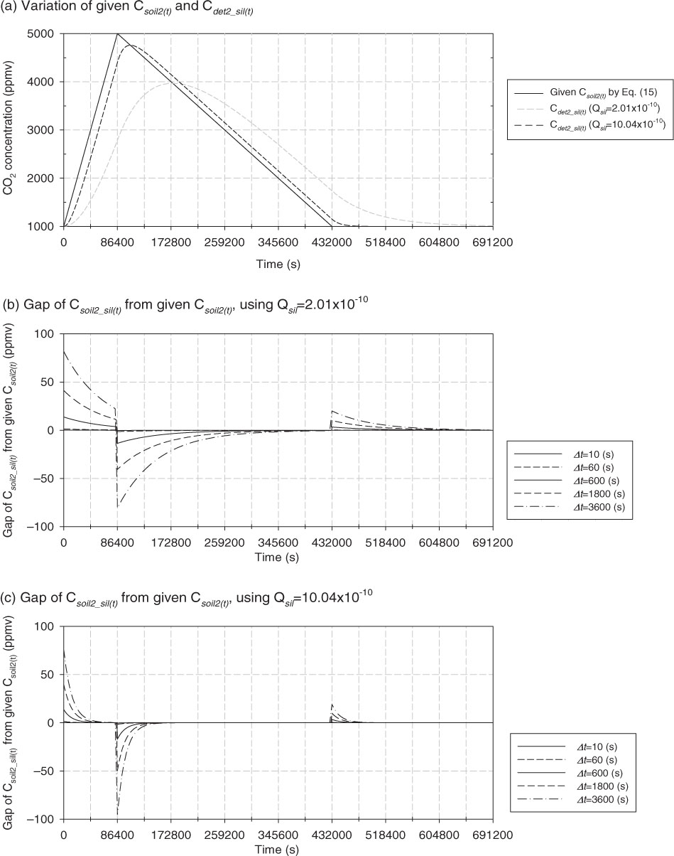
Fig. 3
(a) Time variations of given C soil(t) (black solid line) by eq. (15) and C det_sil(t) with Q sil=2.01×10⁻¹⁰ and 10.04×10⁻¹⁰ mol m m−2 s−1 kPa−1 (grey dashed line and black dashed line, respectively); (b) Time variation of the gap of C soil_sil(t) from given C soil(t), using Q sil=2.01×10⁻¹⁰ mol m m−2 s−1 kPa−1 and eq. (13); (c) Time variation of the gap of C soil_sil(t) from given C soil(t), using Q sil=10.04×10⁻¹⁰ mol m m−2 s−1 kPa−1 and eq. (13). Lines are depicted as Fig. 2.
4.3. Laboratory experiment
The variations of C det_cel(t) and C det_sil(t) are presented for comparison in Fig. 4a. Every time after introducing reference gas, C det_cel(t) and C det_sil(t) had approached the CO2 concentration outside the plastic container (approximately 400 ppmv), which is expected to be true because gas penetrates through epoxy resin adhesive or urethane tube to some degree. As might be assumed, C det_sil(t) lagged C det_cel(t). Hereinafter, C soil_cel(t) and C soil_sil(t) represent the calculated CO2 concentrations in the plastic container. C det(t) depends only on the responsivity of the sensor, as expressed in eq. (12). Therefore, C det_cel(t) was assumed to be calculable from C soil_cel(t) without significant error.
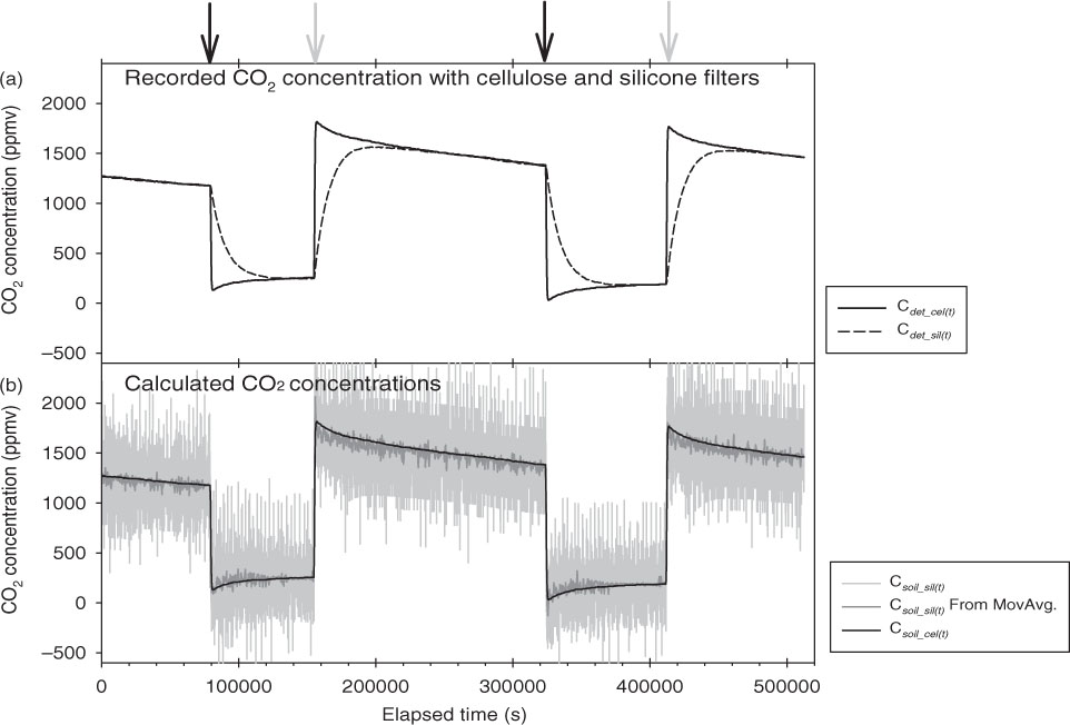
Fig. 4
(a) Time variation of C det_cel(t) (solid line) and C det_sil(t) (dashed line) responding to CO2 concentration in the container. Black and grey arrows respectively indicate the time to infuse the N2 and air-balanced CO2 standard (1930 ppmv) gases; and (b) time variation of C soil_sil(t) (grey line), C soil_sil(t) calculated from 60-data (10 min) moving averages of C det_sil(t) (dark grey line) and C soil_cel(t) (black line). These variations are calculated with Q sil=11.5×10⁻¹⁰ mol m m−2 s−1 kPa−1. Black solid lines do not denote the moving average of the grey solid line. C soil_sil(t) and C soil_cel(t) are calculated with eq. (13).
Q sil was calculated as follows. First, C soil_cel(t) was calculated with obtained C det_cel(t) and eq. (13). Furthermore, treating Q sil as an unknown variable, I assumed that C soil_sil(t), which was calculated from obtained C det_sil(t) and eq. (13), overlaps C soil_cel(t). Finally, I obtained the answer Q sil=11.5×10⁻¹⁰ mol m m−2 s−1 kPa−1 using the least squares method. C soil_sil(t) varied fluctuating with width of about 900 ppmv (grey line in Fig. 4b). If C soil_sil(t) was calculated from the series of 60-data (10 min) moving averages of C det_sil(t), then the fluctuation was settled.
4.4. Field experiment
Figures 5 and 6 present results of field experiments. Observed diurnal variation and increment of CO2 concentration because rainfall is indicated, respectively, in Fig. 5 and 6. Both in Fig. 5 and 6, the belated and gentle increase (and decrease) of C det_sil(t) were observed compared to C det_cel(t). Using the calculated Q sil (=11.5×10⁻¹⁰ mol m m−2 s−1 kPa−1) in Section 4.3, the variation of C soil_sil(t) was synchronised with that of C soil_cel(t). The rate of change in C soil_sil(t) was similar to that in C soil_cel(t), but some gap existed between their absolute values. C soil_sil(t) had some fluctuation, but it was settled by calculation from the series of six-data (60 min) moving averages of C det_sil(t).
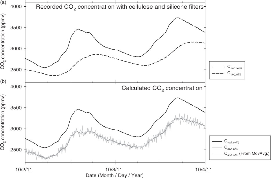
Fig. 5
Observed diurnal variations of CO2 concentration in the field experiment. (a) C det_cel(t) (solid line) and C det_sil(t) (dashed line); (b) C soil_cel(t) (black line), C soil_sil(t) (grey line) and C soil_sil(t) calculated from six-data (60 min) moving averages of C det_sil(t) (dark grey line). These variations are calculated with Q sil=11.5×10⁻¹⁰ mol m m−2 s−1 kPa−1. Black solid lines do not show the moving average of the grey solid line.
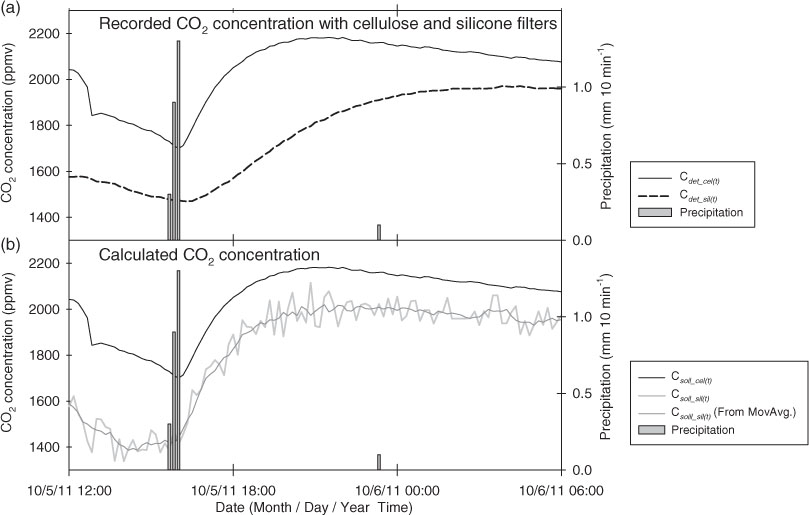
Fig. 6
Observed time variations of CO2 concentration after rainfall in the field experiment. (a) C det_cel(t) (solid line) and C det_sil(t) (dashed line); and (b) C soil_cel(t) (black line), C soil_sil(t) (grey line) and C soil_sil(t) calculated from 6-data (60 min) moving averages of C det_sil(t) (dark grey line). These variations are calculated with Q sil=11.5×10⁻¹⁰ mol m m−2 s−1 kPa−1. Black solid lines do not show the moving average of the grey solid line.
5. Discussions
5.1. Theoretical uncertainty
Strictly speaking, Δt=600 might not be applicable to the equations which lead to C soil(t) under the assumption that Δt is micro time. However, in the case of Δt=600, theoretical calculation indicated that diurnal variation of soil CO2 gas concentration can be evaluated with a silicone-covered CO2 sensor without marked error. Regarding a sudden increase (or decrease) in CO2 gas concentration mainly caused by rainfall event, a silicone-covered CO2 sensor evaluates soil gas CO2 concentration with a larger gap than in the case of diurnal variation. However, the proportion of this gap to the extent of increase was small. The degree of these errors depends on the pattern and scale of the variation, but the reliable variations of CO2 soil gas concentration were revealed by the obtained data.
5.2. Practical application
In field experiments, a gap separating C soil_cel(t) and C soil_sil(t) remained, which might indicate the spatial variation of soil CO2 gas concentration: an unavoidable shortcoming of one-point measurement. In addition to responsivity, it is necessary to tackle this issue.
In both laboratory and field experiments, the variations of C soil_sil(t) were similar to those of C soil_cel(t). The exact gas permeability coefficient, as inferred from laboratory experiments, is indispensable to evaluate the exact variation of soil gas CO2 concentration. Figures 2 and 3 show that the sensor responsivity depends strongly on Q sil. My calculated Q sil is slightly larger than the reference value reported by Lebovits (1966), but my calculated value can be regarded as a plausible value.
The fluctuations of C soil_sil(t) in the laboratory experiment were greater than those in the field experiment. This high level of fluctuation probably occurs because the degree of fluctuation of C det_sil(t) in the laboratory experiment was greater than that in the field experiment. Nevertheless, none of the variations of C det_sil(t) appear to fluctuate in the indicated time scale. This is related to the difference of resolutions between the data loggers. The CR1000 data logger resolution (1333 µV,=1.67 ppmv) in the field experiment was better than that of VR-71 (5 mV=6.25 ppmv) in the laboratory experiment. The notched variation of C soil_sil(t) reflects irregular variation attributable to low resolution of the data logger or sensor. Especially, low resolution of the data logger influenced the fluctuation of C soil_sil(t) in this study. The fluctuation of C soil_sil(t) can be alleviated using a moving average of the recorded data. Application of an approximation curve can also be useful.
6. Conclusions
The following conclusions were inferred from theoretical calculations, and from laboratory and field experiments. The observed variation in the CO2 concentration by silicone-installed sensor in soil is lagged and dampened compared with the real variation. However, the time variation of CO2 concentration in soil was evaluated from the data series obtained using the silicone sensor. For accurate estimation overall, accurate estimation of the gas permeability of silicone is indispensable. A smoothly varying data series should be prepared, which means that a sensor and recording device with high accuracy and resolution must be used. Applying a fitting curve and using a moving average to smooth the obtained data are expected to be useful when using sensors and devices with lower precision. Although the introduced equations and assumptions include some uncertainty, they are available for evaluating the variation of gas CO2 concentration in soil with recorded data every 10 min. The study results demonstrate that silicone-covered diffusive model CO2 sensors are applicable to estimate the time variation of CO2 concentrations in soil.
Acknowledgements
The author expresses his sincere appreciation to the members of laboratory of meteorology in NARO Hokkaido Agricultural Research Centre for providing CO2 sensors and other equipment. The author also thanks Dr. T. Hirota, Mr. T. Hamasaki, Dr. S. Inoue and Dr. M. Nemoto for their useful comments. This work was supported by JSPS KAKENHI Grant no. 23-3318.