
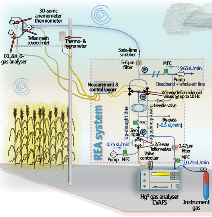
Fig. 1
Schematic representation of the REA-OPEC-measuring complex (not to scale). In the outlined airflow path, MFC denotes a mass flow controller and encircled P indicates the position of a pressure transmitter.
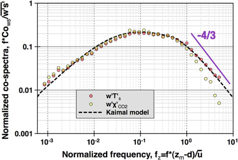
Fig. 2
Cospectra of vertical wind speed (w) with CO2 (yellow filled circles) and sonic temperature, T (red filled circles) based on the daytime data from YCES with unstable conditions. As a reference, the corresponding Kaimal model cospectrum is displayed (dashed curvature) as well as the −4/3 slope (filled purple line) expected from Kolmogorov's theory.
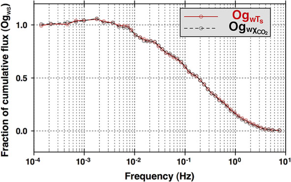
Fig. 3
An ogive calculated for 12:00–14:00, May 10, 2012 at YCES.
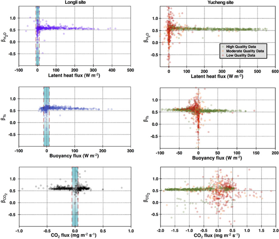
Fig. 4
β-factor () as a function of scalar fluxes over a grassland (left column) and winter wheat stand (right column) fetch. Upper panel: latent heat flux, middle panel: buoyancy flux, lower panel: CO2 flux. In all of the panels, some data are positioned outside the plot range. The data from YCES was segregated into three quality classes based on turbulence tests (see Section 2.3).
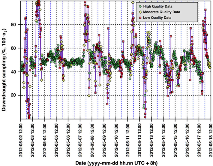
Fig. 5
Daily courses of the distribution () of downdraught sampling with respect to quality indexed groups (high-quality green circles, moderate quality yellow diamond and low-quality red squares).
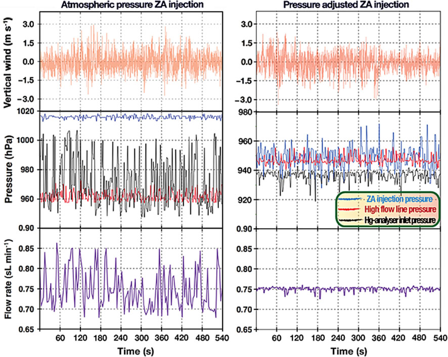
Fig. 6
Characteristics of the REA-CVAFS system without (left column) and with the use of pressure adjusted Hg-zero air injection (right column). For each case, typical time series for daytime unstable conditions are given for w (upper panels, 10 Hz), line pressures (middle panels, 2.5 Hz) and mercury analyser sampling inlet flow rate (lower panels, 1 Hz).
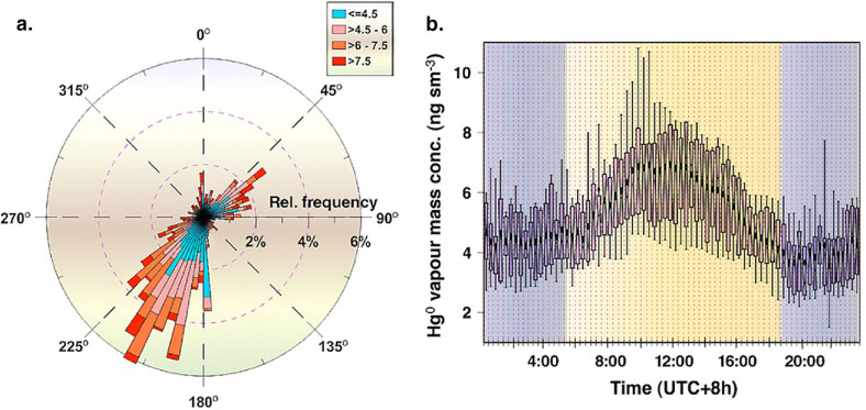
Fig. 7
Polar histogram of 20-minute averaged 5° per bin Hg0 conc. (ng sm−3) classified into four magnitude levels (a. left). Diurnal variation of Hg0 concentrations is represented as a notched box &whiskers percentile plot (b. right). The end of the whiskers represents the 10th and 90th percentile respectively while the half width of the notches is calculated by , where n is the number of samples. Mean is indicated by filled diamonds.
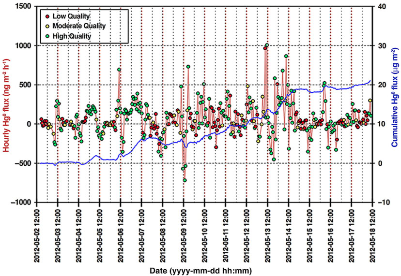
Fig. 8
Time series of 1-hour averaged Hg0 flux (ng m−2 h−1, filled circles with colours based on turbulence quality classes, See Fig. 5) and corresponding cumulative flux (µg m−2, blue solid line) over the experimental period at YCES.
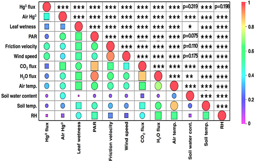
Fig. 9
Heatmap matrix plot of Spearman's rank-order correlation coefficients (ρ) between Hg0 concentration, Hg0 flux and environmental variables. The absolute value of ρ is indicated by a colour code explained in the legend. Circles indicate a positive correlation while square markers represent a negative one. The scale of a marker is proportional to ρ 2. Cells above the matrix diagonal refers to the statistical significance (p) of ρ. Significance levels p<0.05, p<0.01 and p<0.001 are indicated by *, * and *** respectively while a value p ≥ 0.05 is stated explicitly.
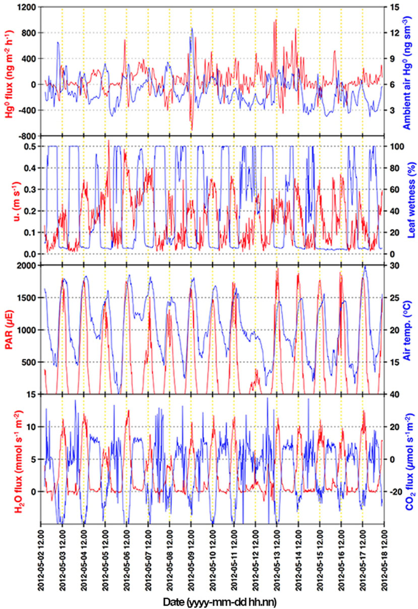
Fig. 10
Time series of selected environmental and meteorological parameters measured at YCES. Panel a: Hg0 flux (red, left) and air Hg0 concentration (blue, right); panel b: friction velocity u* (red, left) and canopy leaf wetness degree (blue, right); panel c: PAR (red, left) and air temperature (blue, right); panel d: H2O flux (red, left) and CO2 flux (blue, right).
{ label needed for table-wrap[@id='T0001'] }
SymbolMeaningUnitTurbulent water vapour flux (measured by EC)g m−2 s−1Turbulent latent heat flux (measured by EC), W m−2Turbulent buoyancy flux (measured by EC)W m−2Turbulent sensible heat flux (measured by EC)W m−2Turbulent carbon dioxide flux (measured by EC)mg m−2 s−1Turbulent elemental mercury vapour flux (measured by REA)ng m−2 h−1Co ws Cospectral density of w and s1Og ws Ogive function1Mass concentration (density) of elemental mercury vapourng m−3c p Specific heat of air at constant pressureJ kg−1 K−1dDisplacement heightmfFrequencys−1f z Normalised frequency−gAcceleration due to gravitym s−2hCanopy heightmLObukhov lengthmPPressurePaP 0 Standard pressure (1013.25 hPa)qSpecific humiditykg kg−1R d The ideal gas law constant for dry airJ kg−1 K−1ReReynolds number–TAir temperatureKT 0 Standard temperature (273.15 K)T s Sonic air temperatureKuLongitudinal component of the wind velocitym s−1u * Friction velocitym s−1wVertical component of the wind velocitym s−1w 0 Magnitude of deadband for REA methodm s−1xHorizontal direction parallel to the average wind velocity/fetchmMean of the scalar x1Predicted value of scalar x1zHeightmz * Height of the roughness sublayermz 0 Roughness height/lengthmz m Measurement heightmaFraction of time of up- and downdrafts to the total sampling time: and respectively.–Relaxation coefficient used in REA measurements without deadband application obtained from OPEC and REA simulations of a specific scalar s–Relaxation coefficient used in REA measurements with a deadband application w0 obtained from OPEC and REA simulations of a specific scalar s–zDimensionless height (z m –d)/L–kVon Kármán's constant (~0.41)–λLatent heat of vapourisation for waterJ kg−1ρSpearman's rank-order correlation coefficient–ρ d Air density (dry)kg m−3σStandard deviation1σ w Standard deviation of vertical wind speedm s−1χ s Mass mixing ratio of scalar component skg kg−11 Dimension according to the use of the parameter.