Fig. 1.
Upper left and lower left panel: Covariance function of vertical wind speed and temperature and covariance function of vertical wind speed and ΣNr concentration measured by the TRANC-CLD system, respectively. Upper right and lower right panel: Normalized flux ogives, i.e. cumulative cospectra of sensible heat and ΣNr flux, respectively. Data were recorded on 7 June 2008, 11:00–11:30 am.
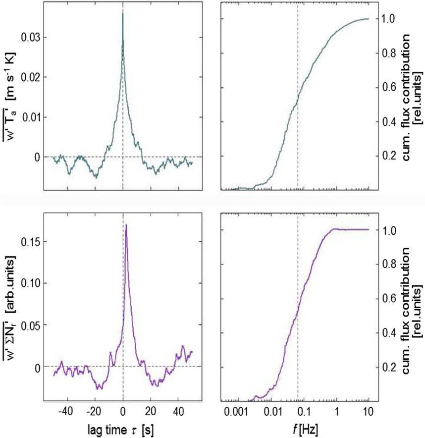
Table 1. Classification of deposition and emission dominated periods during the measurement campaign from December 2007 to November 2008
Fig. 2.
Mineral fertilizer applications (grey bars), field management [harvest (a), tillage (b), and deep tillage with subsequent row forming for potato planting (c)] as well as vegetation height (dark green line) (Panel A), cumulative precipitation (Panel B), daily mean air temperature (red line) and net radiation (black line) (Panel C), half-hourly means of ΣNr concentrations (Panel D), monthly boxplots of ΣNr concentrations with red horizontal lines indicating the median, blue horizontal lines indicating lower and upper quartile values, black whiskers representing the interquartile range and outliers from this range plotted as grey crosses (Panel E), half-hourly means of ΣNr fluxes (Panel F), and monthly boxplots of ΣNr fluxes (Panel G; same colour and line coding as in Panel E) during the observation period from December 2007 to November 2008.
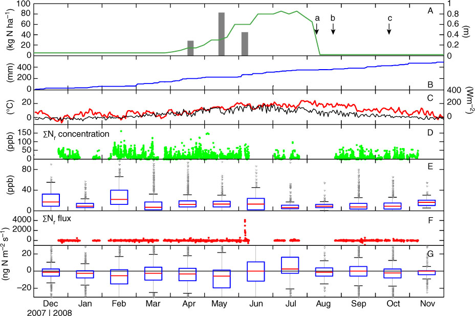
Fig. 3.
Mean diurnal variation of ΣNr concentrations separated in periods dominated by deposition (Panel A) and periods dominated by emission (Panel B). Emission period 3 (E3) was divided into sub-sections due to significant changes four days after fertilization.
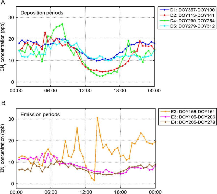
Fig. 4.
Monthly mean concentrations of ΣNr measured by the TRANC-CLD system (red line) and DELTA denuders (blue line) in ppb (left y-axis). Each dot of the DELTA line represents the sum of NH3, HNO2, HNO3, particulate NO3 and particulate NH4. Monthly mean atmospheric stability ς is shown in grey (right y-axis) (Panel A). Panel B shows a map of the Thuringian Basin with the field site in Gebesee and the City of Erfurt. Mean frequency distribution of wind direction for selected periods and mean frequency distribution of ΣNr concentrations measured by the TRANC-CLD system for selected periods are shown in Panel C and Panel D, respectively.
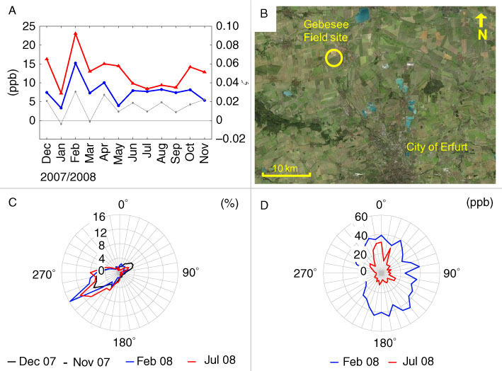
Fig. 5.
Dependency of ΣNr concentration (Panel A), ΣNr deposition fluxes (Panel B), and ΣNr emission fluxes (Panel C) on friction velocity (u * in m s−1). All u * data are from the net deposition period D2 (DOY113–DOY141, cf. Table 1) and are bin-averaged into 0.05 m s−1 classes with the black markers representing the arithmetic mean. Red horizontal lines indicate the median, blue horizontal lines indicate lower and upper quartile values, black whiskers represent the interquartile range and outliers from this range are plotted as red crosses.
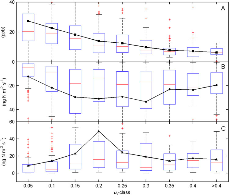
Fig. 6.
Frequency distribution (Panel A) of 30-min ΣNr fluxes from the entire observation period (December 2007 to November 2008). Vertical lines indicate the estimated flux detection limit (σ=3.314 ng m−2 s−1) at −σ and +σ. Panel B shows the cumulative sum of the 30-min ΣNr flux frequency distribution. As indicated by the vertical and horizontal lines, 30.2% of the measured ΣNr fluxes are within the 2σ-sector around zero exchange, i.e. the point where deposition changes to emission or vice versa. Although single flux values were ranging from −166 to 4145 ng m−2 s−1, x-axes are truncated at −110 and +110 ng m−2 s−1 due to only marginal contributions outside these ranges.
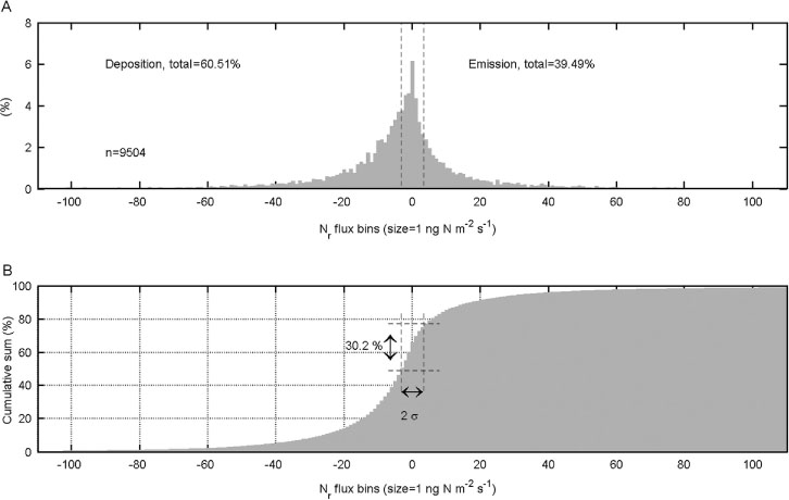
Fig. 7.
Mean diurnal variation of ΣNr fluxes separated in periods dominated by deposition (Panel A) and periods dominated by emission (Panel B). Due to the logarithmic scale, some negative night-time flux values in a range of −50 to 0 ng N m−2 s−1 are missing in Panel B. As for Fig. 3, emission period 3 (E3) was divided into sub-sections by reason of significant changes in exchange characteristics four days after fertilization.
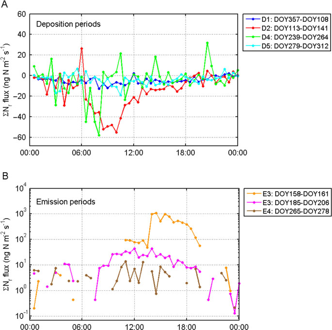
Fig. 8.
Mean diurnal variation of ΣNr concentration (Panel A), ΣNr flux (Panel B), stomatal conductance (g s ) (Panel C), ΣNr concentration multiplied by g s (Panel D), and the dependency of ΣNr flux on ΣNr concentration multiplied by g s (Panel E) during deposition phase D2 (DOY113–DOY141).
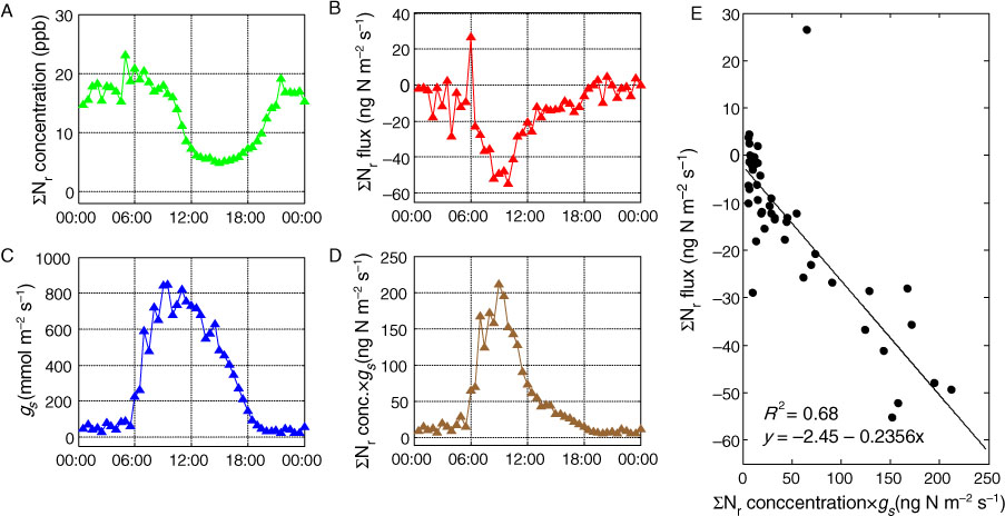
Fig. 9.
Half-hourly ΣNr fluxes following fertilization on 6 June 2008 (DOY158) (Panel A) as well as half-hourly ΣNr fluxes in selected net emission periods before (Panel B) and after harvest (Panel C).
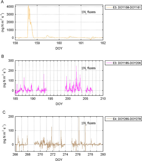
Fig. 10.
Comparison of monthly sums of N exchange as determined by the TRANC-CLD system (black line) and by four inferential models (cf. Flechard et al., 2011), i.e. the UK CBED scheme (CB), the dry deposition module of the Environment Canada model (CD), the surface exchange scheme of the EMEP model used under CLRTAP (EM), and the Dutch IDEM model (ID) (Panel A). Panel B shows the monthly ensemble means of the four models displayed in Panel A with each monthly value being composed of the compounds NH3, HNO3, NO2, particulate NH4, and particulate NO3. Standard deviations of each compound based on these deposition rates are shown in Panel C.
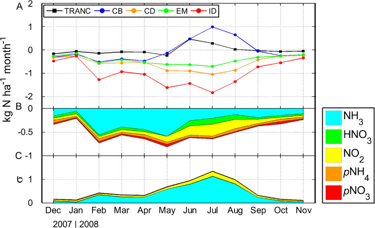
Fig. 11.
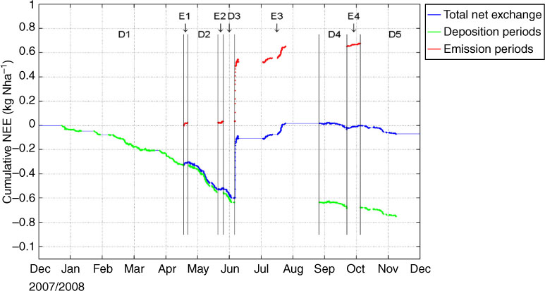
Cumulative net ΣNr exchange during the entire observation period from December 2007 to November 2008. The red line indicates the cumulative net ΣNr loss to the atmosphere during net emission periods, the green line indicates the cumulative net ΣNr gain of the plant–soil system during net deposition periods, and the blue line represents the cumulative total net ΣNr exchange. Periods D1–D5 and E1–E4 correspond to naming in Table 1.