
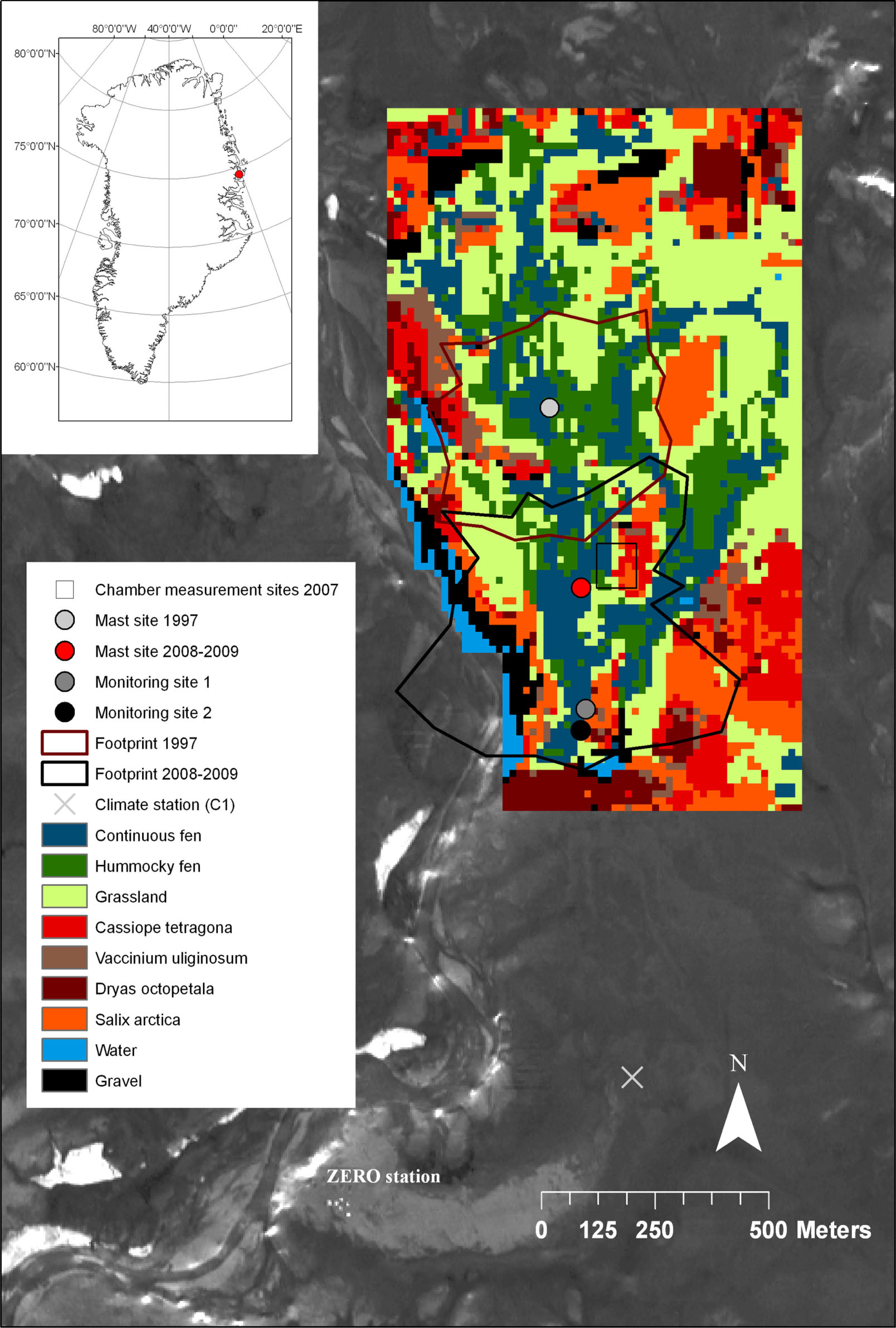
Fig. 1
The Zackenberg valley and the investigation area surrounding the research station (ZERO). The field inventory map of the dominant plant communities estimated in the Rylekærene study site is superimposed over the area. The vegetation map is the studied area referred to as Rylekærene throughout the text. The red dot on the Greenland map is the location of Zackenberg. The Footprint areas are the average 80% cumulative flux distances of the two towers.
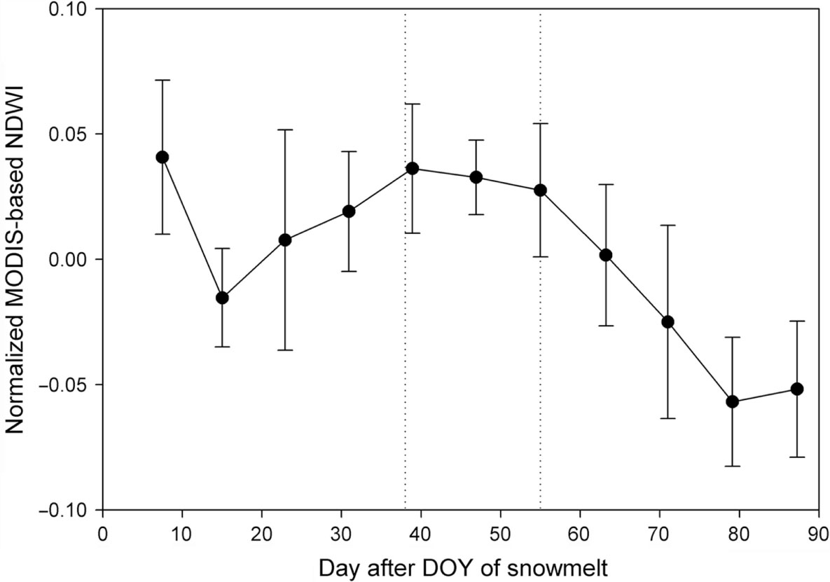
Fig. 2
Average (±1 SD) normalised NDWI based on MODIS surface reflectance data 2000–2010. Data was averaged for each 8-d period after DOY of snowmelt and it was normalised against the seasonal average NDWI. The dotted lines show the time window used for choosing high-resolution Landsat data day 38–55 after DOY of snowmelt.
Table 1
The different sensors recording the Landsat images that were used in the analysis
[i] Day of year (DOY) when the images were obtained is also included. The DOY of 10 cm snow depth for the different years, which was used as start of the growing season, is also given.
[ii] aDOY of 10 cm snow depth based on snow coverage by Buus-Hinkler et al. (2006).
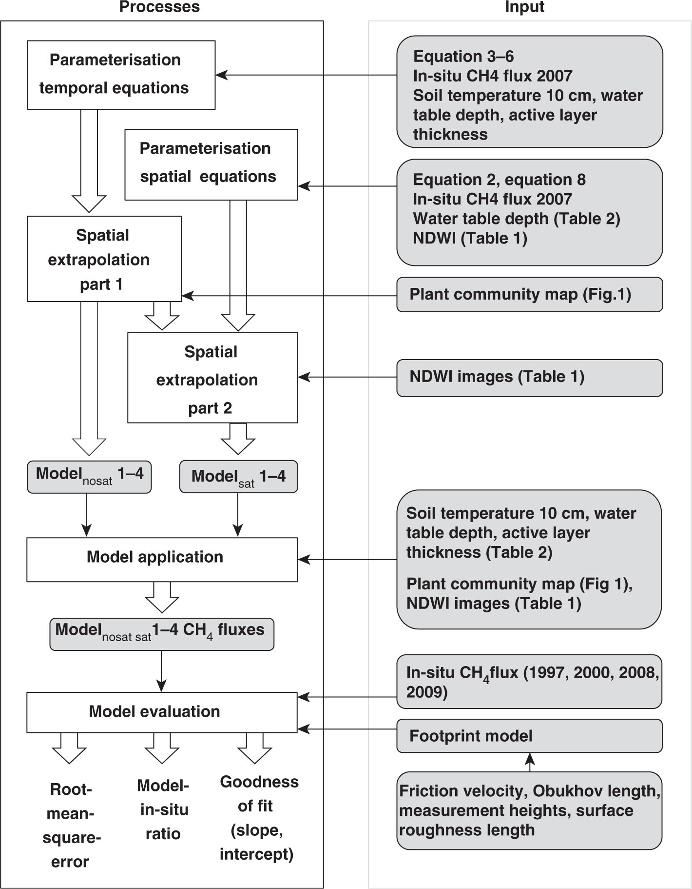
Fig. 3
Workflow for the model development and the model evaluation. The white boxes are steps in the work process of the model development or the model evaluation. The grey boxes are input data or equations going into the models. The thick arrows indicate steps in the work process, whereas thin arrows indicate input. The final results of the model evaluation were the root mean square error, the model-in situ ratio and the goodness-of-fit given by a linear regression equation.
Table 2
Monitored environmental variables used in the modelling of CH4 fluxes
[i] T 10 is the soil temperature at 10 cm depth, WtD is the water table depth and AL is the active layer thickness. Gaps in the data series were filled by linear interpolation. The ‘–’ either means that no measurements were done, or that they were not necessary in the modelling process. M1 is the monitoring site 1, M2 is the monitoring site 2 and T1997 is the Tower site 1997 (Fig. 1).
[ii] a T 10 modelled with a linear regression fitted between T 10 at monitoring site 1 d 1–57 of the growing seasons 2007, 2008 and 2009 and T 10 at C1 (R 2=0.47, n=4147).
[iii] b T 10 was measured from the 8 July 2000. At the start of the growing season, a linear regression fitted between hourly averaged T 10 at monitoring site 2 in 2000 and hourly T 10 at C1 (R 2=0.89, n=1062) was used.
[iv] cAL modelled with a linear regression fitted between AL at monitoring site 1 of the growing seasons 2007, 2008 and 2009 and AL at ZEROCALM1 (Jensen and Rasch, 2011) (R 2=0.96, n=23).
Table 3
Average (±1 SD) CH4 fluxes and environmental variables measured between 10 a.m. and 6 p.m. in the period 30 June–4 August 2007, for the different plant communities
[i] The T 10 is the average soil temperature at 10 cm depth and WtD is the average water table depth (centimetres below moss surface) measured 21 June–4 August 2007. ALmax is the average active layer thickness (centimetres below moss surface) from the 4 August 2007, when the thickest AL was measured.
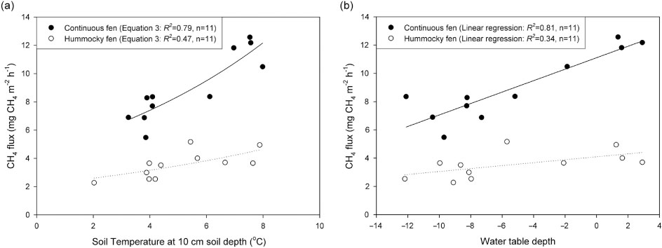
Fig. 4
The relationship between temporal variation in CH4 fluxes to (a) averaged soil temperature at 10 cm depth and (b) averaged water table depth. Equation (3) is given in the text.
Table 4
Parameters for the models relating temporal variation in CH4 fluxes and temporal variation in environmental variables
[i] Linear means a linear regression. Equations (3)–(6) are given in the text. a, b and c are fitted parameters, d was parameterised by Friborg et al. (2000), and R 2 is the coefficient of determination.
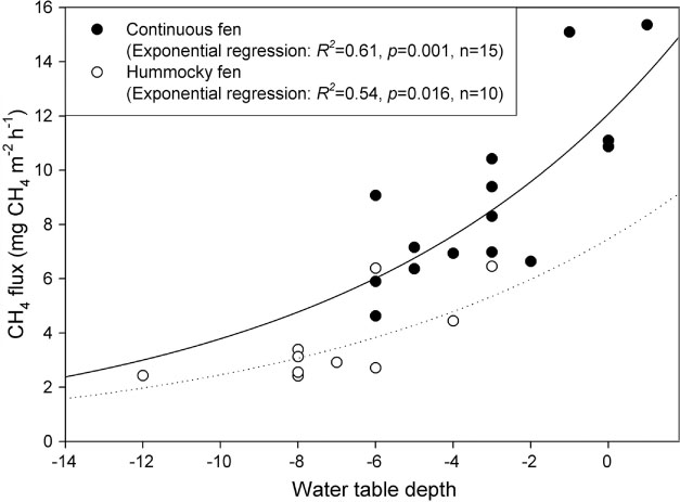
Fig. 5
Plot-averaged CH4 fluxes against spatial variation in water table depth at the DOY of the satellite image 2007 (DOY 210).
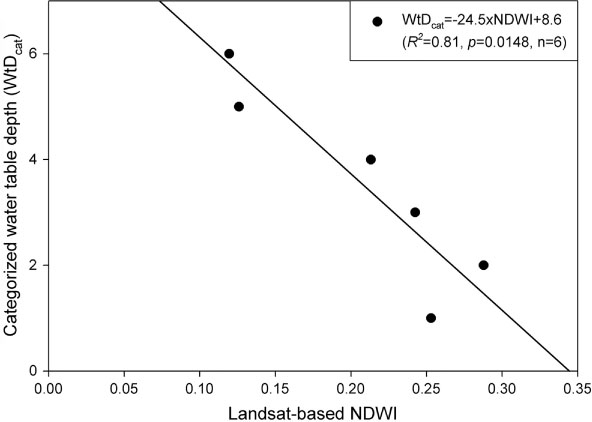
Fig. 6
Categorised water table depth (WtDcat) against Landsat-based NDWI averaged for each WtDcat category. None of the satellite pixels had an average water table above the soil surface, and there is hereby no zero WtDcat.
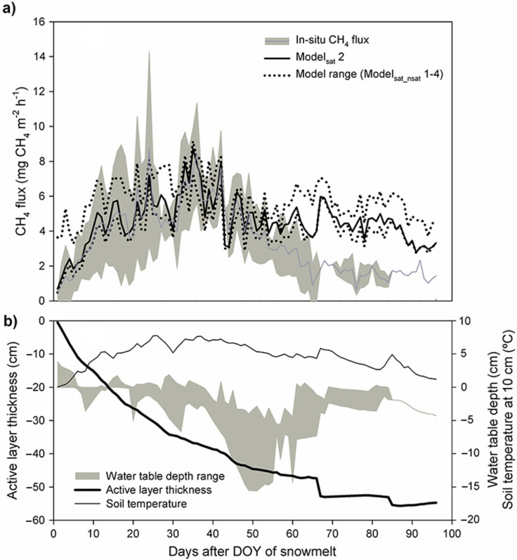
Fig. 7
(a) In situ and modelled CH4 flux and (b) input variables against day after day of year (DOY) of snowmelt. The in situ CH4 flux is the average±1 SD averaged for each day after DOY of snowmelt 1997, 2000, 2007 and 2008. The modelled CH4 flux is the average flux modelled by Modelsat 2 for each day after DOY of snowmelt 1997, 2000, 2007 and 2008. Modelsat 2 was chosen as it was the best model according the model evaluation. The model range is the minimum and the maximum of the eight models averaged for each day after DOY of snowmelt 1997, 2000, 2007 and 2008. The water table depth range is the minimum and maximum of the measured values for each day after DOY of snowmelt 1997, 2000, 2007 and 2008. Active layer thickness and soil temperature at 10 cm depth is the average for each day after DOY of snowmelt 1997, 2000, 2007 and 2008.
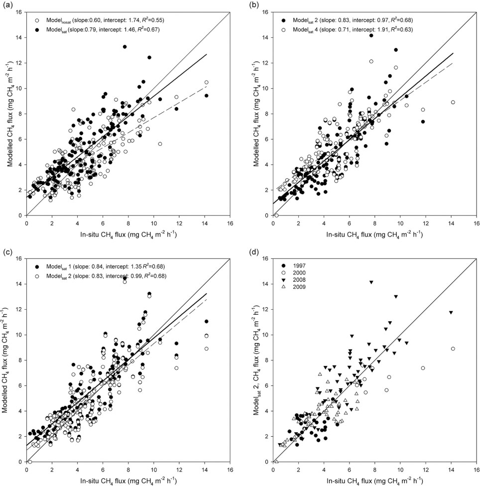
Fig. 8
Modelled CH4 fluxes against in situ CH4 fluxes. (a) Average of modelled CH4 fluxes for all Modelnosat and Modelsat to show the difference between models with and without satellite-based NDWI; (b) Modelsat 2 and Modelsat 4 against in situ CH4 fluxes to illustrate the difference between models including and excluding the temporal variation in WtD; (c) Modelsat 1 and Modelsat 2 against in situ CH4 fluxes to illustrate the difference between models including or excluding the effect of AL; and (d) Modelled CH4 fluxes modelled with Modelsat 2 for the different years against in situ CH4 fluxes.
Table 5
Ratios of modelled CH4 fluxes to in situ CH4 fluxes for the different years and the different models
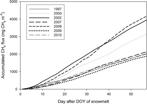
Fig. 9
CH4 fluxes modelled by Modelsat 2, averaged for the Rylekærene area, and accumulated over the first 57 d of the growing seasons 1997–2010.
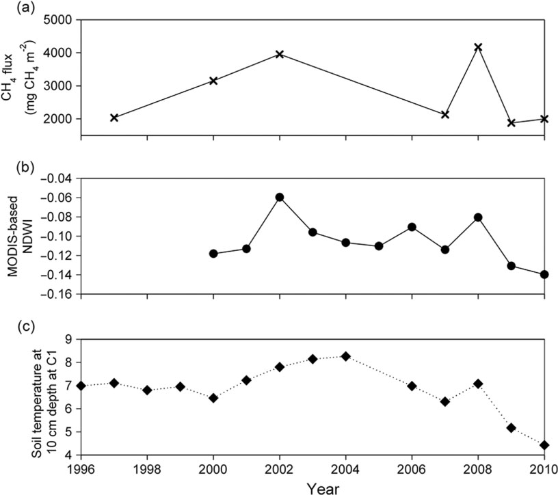
Fig. 10
(a) Accumulated modelled CH4 fluxes day 1–57 of the growing season for Rylekærene; (b) maximum MODIS-based NDWI for the NDWI peak period of the growing seasons in Rylekærene 1997–2010; and (c) and average soil temperature at 10 cm soil depth at C1 day 1–57 of the growing season. The gap in the soil temperature 2005 was caused by broken soil temperature sensors.
Table 6
Average (± 1 model SE) modelled CH4 fluxes for the entire Rylekærene area for the first 57 d of the growing season
Table A
Abbreviations, symbols and their descriptions