A long-term study of aerosol modulation of atmospheric and surface solar heating over Pune, India

1. Introduction

Numerous studies, in the recent past, have highlighted the implications of aerosols on weather and climate. Despite the efforts, the uncertainty remains in assessing their true climatic effects. This is largely due to their spatial heterogeneities/variability (IPCC, 2007). Aerosol, although very small in size (sub-micron and micron-sized particles suspended in air), pose serious challenges to achieve accurate modelling projections of the future climate of our planet. The difficulty in accurately model the effects of aerosol on the Earth's radiative balance is also due to the fact that their properties, such as size distribution, single scattering albedo, asymmetry factor and so on, have shown large variability from region to region over the globe.

Analysis of long-term records of surface solar radiation, either in clear-sky and/or all-sky conditions, suggests significant trends during past decades (Wild et al., 2005; Pinker et al., 2005; Padma Kumari and Goswami, 2010; Soni et al., 2011). The results suggest that such trends result from decadal changes of aerosols, particularly anthropogenic, and an interplay of aerosol direct and indirect effects (Wild et al., 2005; Padma Kumari and Goswami, 2010). However, reliable observations of aerosol trends are needed before these speculations can be proven (Devara et al., 2002). In addition to the aerosol optical depth, we also need to quantify changes in aerosol characteristics/composition because of changes in industrial practices, environmental regulations, and biomass burning emissions which will affect the aerosol single scattering albedo and size distribution, which in turn will affect surface solar radiation. Currently such comprehensive data sets are sparsely available over the globe.

Many investigations have been conducted to characterise atmospheric aerosols and their radiative effects around the world, as recently reviewed by Yu et al. (2006). Studies focusing on Asia include, among others, the Indian Ocean Experiment (INDOEX) (Ramanathan et al., 2001b), the Asian Pacific Regional Aerosol Characterization Experiment (ACE-Asia) (Huebert et al., 2003), the Asian Atmospheric Particle Environment (APEX) (Nakajima et al., 2003), the East Asian Study of Tropospheric Aerosols: An International Regional Experiment (EAST-AIRE) (Li et al., 2007) and cloud-free aerosol radiative forcing across China (Li et al., 2010). In recent years, many studies have been undertaken to assess the impact of aerosols on the climate in the Indian region (Satheesh and Ramanathan, 2000; Ramanathan et al., 2001b; Moorthy et al., 2005; Ramachandran, 2005a, 2005b; Tripathi et al., 2005; Ganguly and Jayaraman, 2006; Pant et al., 2006; Niranjan et al., 2007; Babu et al., 2007; Sreekanth et al., 2007; Dey and Tripathi, 2008). However, a few long-term (5-yr or so) studies have been carried out, whereas most of the other studies are limited in observations span. Also, barring only one long-term study (Dey and Tripathi, 2008), none has utilised columnar measured properties (such as SSA and asymmetry factor) in computing aerosol radiative forcing. In this context, the current measurements and study of the aerosol properties and its impact on climate through radiative forcing from an urban region assumes significance as this may provide benchmark information on the measurement over the tropical (Pune) region.

2. Instrumentation and methodology

Aerosol direct radiative forcing (ADRF) computation is performed by using aerosol parameters pertaining to Pune, a tropical fast growing urban location in India. The details regarding location, local meteorology and instrumentation and so on are available in a paper by Kumar et al. (2011). However, a brief description is given here.

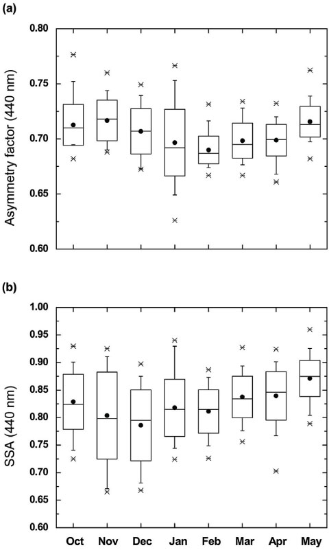
A CIMEL Sun/sky radiometer was installed at IITM (Indian Institute of Tropical Meteorology), Pune, India, in October 2004 as a part of the Aerosol Robotic Network (AERONET) (Holben et al., 1998). Aerosol optical depth (AOD) at 440, 675, 870 and 1020 nm, with an uncertainty of ~0.01–0.02, can be derived from direct radiance measurements (Eck et al., 1999). The measurements at 940 nm are used for the derivation of the water vapour column amount (Alexandrov et al., 2009). The aerosol size distribution, refractive index, and single scattering albedo are retrieved from the sky radiance measurements and AODs at 440, 675, 870, and 1020 nm (Dubovik and King, 2000; Dubovik et al., 2006). The AERONET data employed in the present study belong to the Version 2.0 at level 1.5 (from October 2004 to April 2007) and at level 2.0 (from January 2008 to May 2009), which are cloud-screened and have been further screened manually to ensure the data quality. Figure 1 (a, b) apprises of the range and variability of aerosol optical parameters observed during 5-yr period. The variation in other parameters such as AOD, columnar water vapour, Ångström exponent and volume size distribution has been recently reported in another paper by Kumar et al. (2011). In these box diagrams, the mean is represented by a solid dot. The divisor segment in the box is the median. The top/bottom of each box represents the monthly mean plus/minus the standard deviation. The box bars (whiskers) denote the percentiles 5% and 95%, percentiles 1% and 99% and minima maxima represented by the crosses and dash sign. The in-depth discussion about each of aerosol parameters and transport patterns can be found in a companion paper by Kumar et al. (2011).

Fig. 1. 

2.1. Aerosol radiative forcing

Aerosols modify incoming solar and outgoing infrared radiation. Change in radiation flux caused by aerosol is referred to as aerosol radiative forcing. The effect of aerosol on TOA (which is considered to be about 100 km in this study) radiative fluxes is called TOA radiative forcing and that on surface fluxes is called the surface radiative forcing. The difference between the two is the atmospheric radiative forcing. In all cases (i.e. surface, atmosphere and TOA), aerosol forcing is the difference in radiative fluxes with and without aerosols.

By definition, the aerosol direct short-wave (solar) radiative forcing (ADRF) is the change (ΔF) in the radiation flux (F) either at the surface (S) or at the TOA, respectively without and with the aerosol particles in the atmosphere (Russell et al., 1999; Podgorny et al., 2000; Yu et al., 2001; Pandithurai et al., 2004). This is generally represented as:

1

where F_NA and F_A, respectively, correspond to the short-wave fluxes without and with aerosols, and the subscripts S and TOA refer to the Earth's surface and top of the atmosphere, respectively. The arrows indicate the direction of the fluxes: ↓ downward flux and ↑ upward flux. A negative value of ΔF _TOA implies that the presence of aerosols results in increase in the radiation loss to the space (by enhanced backscattering) leading to a cooling in the Earth-atmosphere system, while its positive value implies an atmospheric warming. At the surface, the aerosol forcing (ΔF _S) will always be negative because aerosols reduce the surface reaching solar radiation.

The difference between the radiative forcing at the TOA (which is 100 km in this case) and the surface is defined as the atmospheric forcing (ATM) and can be written as:

2

where ΔF _Atm represents the amount of energy trapped within the atmosphere due to the presence of aerosols. If ΔF _Atm is positive the aerosols produce a net gain of radiative flux to the atmosphere leading to a heating (warming), while negative ΔF _Atm indicates net loss and thereby cooling.

In the current study, the radiation code SBDART developed by Ricchiazzi et al. (1998) is used to perform radiative transfer calculations in the short-wave (0.3–4.0 µm) region. SBDART is a radiative transfer model which computes plane-parallel radiative transfer both in the clear and cloudy sky conditions within the Earth's atmosphere and at the surface. However, in the present study, all radiative transfer computations are performed for clear sky. The model is well suited for a wide variety of problems in atmospheric radiative energy balance and remote sensing studies. For the molecular absorption part, SBDART uses the low-resolution band models of LOWTRAN-7 atmospheric transmission code. These band models take into account the effects of all radiatively active molecular species found in the Earth's atmosphere and have wavelength resolution of about 5 nm in the visible and about 200 nm in the thermal infrared. In SBDART, radiative transfer equations are numerically integrated using DISORT radiative transfer module developed by Stamnes et al. (1988). The intensity of both scattered and thermally emitted radiation can be computed at different heights and directions. Presently, SBDART is configured to allow up to 65 atmospheric layers and 40 radiation streams (40 zenith angles and 40 azimuthal modes).

The main input parameters required in SBDART include aerosol optical depth, single scattering albedo (ω) asymmetry factor (g), surface albedo, columnar ozone and columnar water vapour. Here, the monthly mean values of these parameters are used. The short-wave aerosol radiative forcing (ARF) calculations are performed using eight radiation streams at 15 min interval for a range of solar zenith angles and 24 h averages are obtained.

The albedo of Earth, i.e. the fraction of the global incident solar radiation that is reflected back to space, is a fundamental parameter of global energy balance (Wielicki et al., 1995, 2005). The Surface albedo required for calculation of ADRF over Pune is obtained from MODIS BRDF/albedo operation product MOD43B3 (Schaaf et al., 2002). MODIS provides both black-sky albedo (directional hemispherical reflectance, BSA) and white-sky albedo (bi-hemispherical reflectance, WSA) at seven spectral bands (0.47, 0.555, 0.659, 0.858, 1.24, 1.64 and 2.1 µm) and the three broadband (0.3–0.7, 0.7–5.0 and 0.3–5.0 µm). Black-sky albedo (BSA) is defined as albedo in the absence of a diffuse component and is a function of the solar zenith angle. White-sky albedo (WSA) is defined as albedo in the absence of a direct component when the diffuse component is isotropic. BSA and WSA mark the extreme cases of completely direct and completely diffuse illumination (Strahler et al., 1999). Actual albedo is a value which is interpolated between these two as a function of the fraction of diffuse sky fraction; which itself is a function of aerosol optical depth (http://www-modis.bu.edu/brdf/userguide/albedo.html). Actual albedos for different months during October 2004 to May 2009 are obtained using the following relation:

3

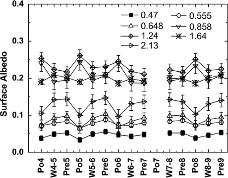
where DSF is diffuse sky fraction which is a function of aerosol loading and solar zenith angle. Observed mean AOD for each month is used to derive DSF using a look-up table provided by MODIS land team. Figure 2 shows the seasonal (averages of corresponding monthly values) variation of surface albedo over Pune, obtained by MODIS at seven different wavelength bands for the period from 2004 to 2009. Vertical bars in this figure represent ±1σ variation about the mean value of surface reflectance measured during that season. On an average, surface reflectance values are found to be higher during pre-monsoon and winter seasons while they are low during post-monsoon season.

Fig. 2. 

The computed aerosol forcing values always involve certain error due to the random (statistical) error of the input parameters of the model. The resulting uncertainty of the aerosol forcing value is estimated here by the method of error propagation (Feczko et al., 2005). While discussing the implications of the temporal variations of radiative forcing due to aerosols, it is important to account for the error budget for such estimations. The source and magnitude of the uncertainties will indicate the current status of the required data and future needs and help in comparing with other estimations globally. The quality of aerosol optical properties determines the accuracy of the estimated ADRF. Table 1 shows the percentage change in aerosol forcing values with respect to given uncertainties in input variables. The uncertainties associated with input parameters: aerosol optical depth, single scattering albedo, asymmetry factor and surface albedo are ±0.02, ±0.03, ±0.05 and ±10%, respectively (Dubovik et al., 2002; Xia et al., 2007). The resulting errors in the estimates of ADRF (surface and TOA) are estimated on the basis of the uncertainty ranges of input variables such as AOD, SSA, asymmetry factor and surface albedo. The net error is the difference between the flux calculated with and without the error in the parameter under study against that calculated for the reference values of input parameters. The effects on the ADRF at the surface (ADRF_S), varying from about 0.7% to 6.1%, are less pronounced compared to the effects on the ADRF at the TOA (ADRF_TOA), which range from 14.3% to 44.6%. The effect of aerosol scattering and absorption on ADRF is dominant. The large differences in percentage changes may be attributed to the fact that TOA radiation flux is affected by outgoing radiation only (since incoming flux at TOA is same for both aerosol and non-aerosol cases), whereas at surface it is a function of incoming as well as outgoing flux. Considering that the input parameters are independent (Xia et al., 2007), we may estimate the overall error in the calculated ADRF due to uncertainties in the input parameters as:

Table 1. Percentage change in aerosol direct radiative forcing at the surface (ADRF_SUR) and at the top of atmosphere (ADRF_TOA) due to uncertainties involved in aerosol optical depth (τ), single scattering albedo (ω), asymmetry factor (g) and surface albedo (a).

τωga ΔADRF_SUR 6.1% 5.6% 3.2% 0.7% ΔADRF_TOA 14.3% 39.5% 44.6% 19.1%

2.2. Comparison between measured and calculated fluxes

The ability of the SBDART model to predict clear-sky diffuse and global broadband short-wave irradiances is investigated. Model calculations of these quantities are compared with data obtained from surface-based instruments. The measurements of global and diffuse surface fluxes were made simultaneously by two identical (shaded and unshaded) instruments. The flux data was screened to eliminate the effects of clouds.

Two pyranometers (one shaded and the other unshaded) were installed at the IMD (India Meteorological Department) Pune radiation lab. They were in operation for more than 20 yr. Thermoelectric pyranometers were utilised to acquire the radiation data in the wavelength range from 0.3 to 3.0 µm. The absolute accuracy of the standard instrument is about ±0.3%, while the accuracy of the instruments in the network is about ±2% (Soni et al., 2011), and the data generated in the network are well within the accuracy limits specified by World Meteorological Organization (1983). The hourly data set, from October 2004 to December 2008, was utilised for comparison.

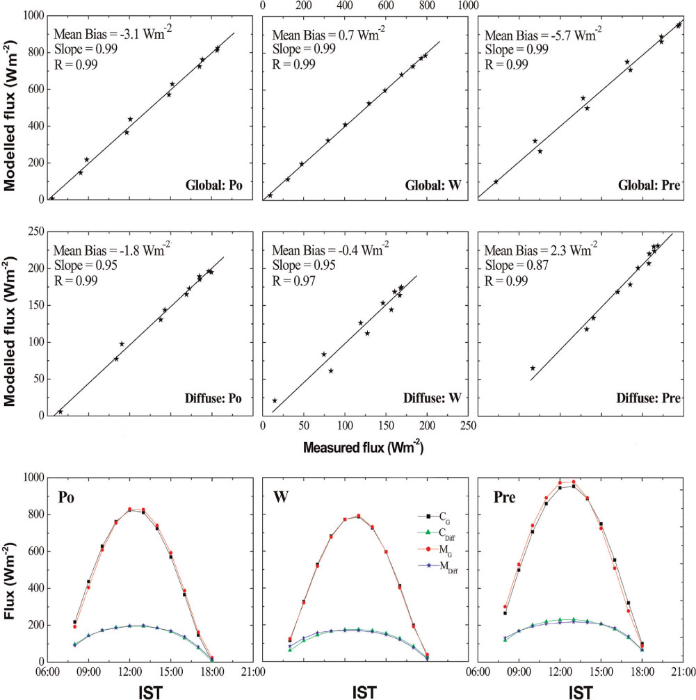
The clear-sky day data from October 2004 to December 2008 were averaged discretely for each season. The seasonally averaged global and diffuse irradiances calculated from SBDART were used for comparison, separately, with the surface-measured irradiance values. Shown in Fig. 3 are measured global (top panel), diffuse fluxes (middle panel) plotted as a function of calculated flux and their average diurnal (bottom panel) variation, at the surface. The measured and calculated global fluxes are in very good agreement with the mean bias of −3.1, 0.7 and 5.7 Wm⁻²; slope of 0.99, 0.99 and 0.99, for post-monsoon, winter and pre-monsoon respectively. Similarly, measured and calculated diffuse fluxes are also found to agree well with mean bias of −1.8, −0.4 and 2.3, for post-monsoon, winter and pre-monsoon respectively. Here mean bias represents the average difference between calculated and measured fluxes. The slope is calculated using the least square fitting. A potential source of difference between calculated and measured fluxes is the uncertainty in the flux measurements (~±5Wm⁻²). Nevertheless, there is a good correlation among flux values. Good agreement between the measured and modelled down- welling fluxes (global and diffuse) demonstrates that the input parameters, particularly the retrieved aerosols properties, reasonably represent atmospheric conditions over the experimental site.

Fig. 3. 

3. Aerosol direct radiative forcing

Radiative forcing due to aerosols are estimated by taking differences of results obtained by running the radiative transfer model with and without aerosol loading in the atmosphere under clear-sky conditions. Calculations of radiative fluxes integrated over the entire short-wave region for all atmospheric layers are carried out at every 15 min interval and for a 24-h period. In this section, the monthly mean climatology and the inter-annual variations of ADRF in clear-sky condition over Pune are discussed.

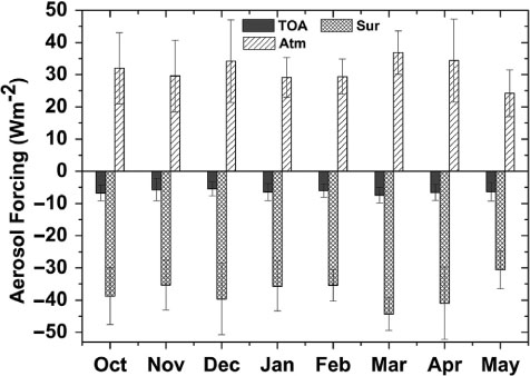
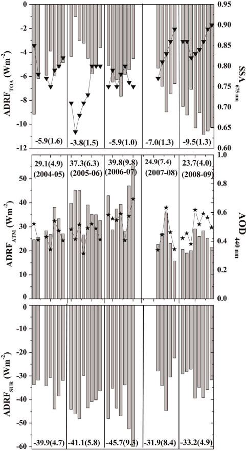
Figure 4 shows the average values of short-wave ADRF at the surface level and TOA for the period from 2004 to 2009. Radiative forcing calculations have been carried out separately for each month in all years. The annual (annual here denotes the period from October through May, since it is not possible to make any reliable observations over Pune during monsoon season spanning 4 months, June to September) mean surface, TOA and atmospheric clear-sky forcing over Pune are −37.7±8.2, −6.4±2.4 and 31.3±9.1 Wm⁻², respectively. Large negative surface forcing (more than −30 Wm⁻²) is observed in all the months with three peaks, during October, December and March months when the surface forcing exceeds approximately −40 Wm⁻². Surface forcing values are higher for pre-monsoon months, comparable for winter and post-monsoon months. The TOA forcing is found to be negative for all months with minor variations. The difference between the TOA and surface-level forcing is taken as atmospheric forcing. It represents the amount of energy trapped within the atmosphere by aerosols and mostly results in heating of the atmosphere (Ramanathan et al., 2001b). Atmospheric forcing will increase if aerosol forcing at the TOA is more toward positive side while there is a large negative forcing at surface level. Figure 4 portrays that very high atmospheric heating (more than 20 Wm⁻²) persists throughout the year. These interactions between aerosols and solar radiation can be attributed to combination of aerosol properties (loading, optical properties, size distribution, shape), surface properties (e.g. spectral variations of surface albedo), and geographical parameters (latitude, season) (Yu et al., 2006).

Fig. 4. 

Trapping of energy in the atmosphere, due to large differences between the TOA and surface forcing, is of great importance to know how this heating is distributed within the atmosphere. This is also useful to understand how various components of the Earth-Atmosphere system could respond to such large-scale heating perturbations. As discussed by Kumar et al. (2011) and observed in Fig. 1, large variability exists in the aerosol loading, their optical properties during different months/seasons of the year. In addition to these, there are large monthly/seasonal differences in meteorological parameters (the important one being the distribution of water vapour in the atmosphere) and even reflectance of the underlying surface (Fig. 2). The temporal variations of clear-sky ADRF, shown in Fig. 5, will describe how these factors contribute to effect different values of radiative forcing in the atmosphere. It is interesting to note that the monthly variations of ADRF over Pune in each year are not similar. There is a large negative forcing at the surface level in the range of −22 to −60 Wm⁻², while forcing at TOA varied between −1.0 and −11 Wm⁻². Atmospheric forcing, which is difference between TOA and surface forcing is the absorption within the atmosphere is very large over this region (varied from 15 to 55 Wm⁻²). The middle and lower panel of Fig. 5 shows that the surface and atmospheric level radiative forcings are primarily governed by the magnitude of AOD values which varied mostly between 0.3 and 0.7 at 440 nm during 2004 to 2009. Whereas the TOA seems to be intricately dependent on several aerosol parameters, such as AOD, surface albedo, SSA and so on. Negative values of ADRF at the TOA over the study region and its increasing or decreasing trend seems to be closely associated with SSA values. This implies that more of the scattering type of aerosol (large SSA values) leads to more negative TOA forcing values, i.e. more radiations are leaving the top of atmosphere.

Fig. 5. 

4. Comparison and implications to regional climate

In the previous sections, the temporal variability of the ADRF over Pune region has been discussed. Comparison of these values with those estimated over other polluted regions in India, neighbouring countries and pristine (oceanic) regions around the Indian subcontinent is of great interest. In order to investigate these issues, a comparative study is made with the available estimates from literature. The regions are characterised on the basis of kind and strength of sources. The ADRF values for Pune are compared with the estimates made for other polluted cities in India and adjoining regions in Table 2.

In India, besides Pune, only at a few places ADRF has been estimated. But, still the stations which employ columnar measured properties like SSA, asymmetry factors are less in number than those use surface-level measurements to derive these properties to compute ADRF. All mainland stations show higher atmospheric absorption, with more or less comparable values, on annual/seasonal scale in comparison to adjoining oceans. It is seen that the TOA forcing was mostly negative at Trivandrum, whereas it was positive over Visakhapatnam for all the seasons. It is negative during winter and retreating monsoon and positive during pre-monsoon and monsoon seasons over Ahmedabad. The magnitude of TOA forcing, observed over Pune, is more or less comparable, albeit with a change in sign at some locations. Except for Ahmedabad and Delhi, TOA values are observed to be significantly lower (negative/positive/both) at all other locations. The magnitude of TOA negative values is successively higher for Beijing, the Arabian Sea, the Bay of Bengal and Ahmedabad (except pre-monsoon and monsoon). The higher negative value represents more cooling, i.e. more radiation leaving the top of atmosphere; or the number of scattering type aerosols in the atmosphere of these regions is large.

In Delhi and Ahmedabad, the surface and atmospheric ADRFs are higher than those in Pune because of higher aerosol loading. The surface ADRF seems to be significantly lower at Nainital (high-altitude), Kathmandu, Vishakhapatnam and Bangalore than Pune. ADRF at, Pune, Ahmedabad, Delhi, Dibrugarh, Trivandrum and Kanpur shows higher values as compared to the other locations in India and neighbouring oceans. This could be due to (1) geographic position of the site, (2) prevailing meteorological conditions, particularly the large-scale circulation systems that vary over different study regions from season to season, and influence differently on the aerosol production/removal mechanisms, and (3) continuous source of anthropogenic aerosols throughout the year in association with natural aerosol (sea salt and dust) transported, through long-range transport processes, from oceanic and arid regions in the west. The range of forcing values observed over adjacent countries like China, Korea and Taiwan exhibits almost closer to those observed over Indian mainland and adjoining oceanic regions.

There are a number of factors that cause observed deviations in atmospheric forcing over Pune with other locations of India, such as emissions, column abundance, removal processes, atmospheric transport, optical properties, and physical climate characteristics. The seasonal and spatial variations in ARF and heating rate over the mainland and oceanic regions surrounding India will be useful in the radiative and climate impact assessments. Spatial variability in aerosol characteristics could be the main factor for such variability in forcing estimation.

Minor differences can be seen in estimated forcing values between the present study and the previous one by Pandithurai et al. (2004). In order to ascertain the differences, we performed an exercise for the same months (November to April) by putting the uniform albedo value (0.15), as the case with previous study, in the model instead of wavelength dependence of albedo and found that the present values fall short by 9% and 85% at surface and TOA levels, respectively. Thus, this explains differences.

4.1. Atmospheric heating

The radiative and subsequently the climate implications of aerosols are assessed in terms of the atmospheric heating rate. The atmospheric forcing in Wm⁻² [eq. (2)] indicates the amount of radiative flux (energy) absorbed by aerosols. High short-wave atmospheric forcing values imply that the excess energy in this region is trapped in the atmosphere. According to Liou (2002) the heating rate of the atmosphere is:

4

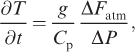
where is the heating rate, C _p is the specific heat capacity of air at constant pressure, ΔF _atm is the atmospheric heating, g is the acceleration due to gravity and ΔP is the atmospheric pressure. A major amount of aerosols is present in the lower level, i.e. up to the height of boundary layer, and contributes to atmospheric heating; hence, altitude is taken as 3km (e.g. Ramanathan et al., 2001b; Lubin et al., 2002; IPCC, 2007). Therefore, ΔP [in eq. (4)] is considered as 300 hPa, which is equal to the pressure difference between surface and 3 km.

The maximum heating of the atmosphere is noticed during pre-monsoon season which is followed by post-monsoon and winter seasons in the decreasing order with their values being 0.94±0.30, 0.86±0.29 and 0.84±0.16 K/day, respectively. Table 3 presents the seasonal variation of atmospheric heating rates over Pune. Heating rate is the highest during pre-monsoon season, because of higher aerosol concentration. Higher values of heating rate in the atmosphere during pre-monsoon season could be due to presence of an elevated aerosol layers during this season (see Kumar et al., 2011). This elevated aerosol layer is largely constituted by dust transported over the measurement location from distant places like northwest India and Arabia besides the locally produced black carbon aerosols which get lifted to higher altitudes because of convective circulation in the atmosphere. This heating in the atmosphere during pre-monsoon seasons can have large implications for the regional climate. Ackerman et al. (2000) have shown that the atmospheric heating by absorbing aerosols can evaporate some of the low-level clouds, resulting in a decrease in cloud cover and planetary albedo. The seasonal changes in heating rate resemble that of seasonal variations in AOD indicates their strong affinity. Ganguly and Jayaraman (2006), Babu et al. (2007), Sreekanth et al. (2007), and Dey and Tripathi (2008) have reported heating rate over Ahmedabad, Trivandrum, Visakhapatnam, and Kanpur to be 0.6–1.13, 0.62–1.51, 0.09–1.23 and~1 K/day respectively, for different seasons. The seasonal heating rate differs from place to place depending on abundance of aerosols, seasons, location, underlying surface, and so on.

Table 3. Seasonal mean aerosol radiative forcing at the surface (SUR), top of the atmosphere (TOA), and in the atmosphere (ATM), along with the heating rate over Pune

Seasons SUR TOA ATM Heating rate, K/d Post-monsoon 2004 −32.76 −7.67 25.09 0.70 Post-monsoon 2005 −45.13 −2.67 42.46 1.19 Post-monsoon 2006 −41.62 −5.79 35.83 1.01 Post-monsoon 2008 −28.68 −8.88 19.81 0.56 Winter 2004–05 −32.43 −4.90 27.53 0.77 Winter 2005–06 −40.50 −3.58 36.92 1.04 Winter 2006–07 −41.46 −6.59 34.87 0.98 Winter 2007–08 −31.02 −6.07 24.95 0.70 Winter 2008–09 −33.81 −8.80 25.01 0.70 Pre-monsoon 2005 −38.16 −5.33 32.83 0.92 Pre-monsoon 2006 −39.11 −4.83 34.27 0.96 Pre-monsoon 2007 −56.23 −4.98 51.24 1.44 Pre-monsoon 2008 −32.51 −7.68 24.83 0.70 Pre-monsoon 2009 −35.53 −10.56 24.97 0.70

The most important implication for high negative surface forcing is the persistent large reduction of direct solar radiation in the Pune and other regions (Table 2). As the insolation at the surface is controlled by aerosols and clouds, the presence of clouds can increase/decrease the surface cooling to some extent in addition to aerosols. Dey and Tripathi (2008) have observed over Kanpur that clouds themselves induce large cooling, two to three times higher than the clear-sky condition. In another study by Ramanathan et al. (2001a), it has been shown that the large surface cooling and atmospheric heating can affect the regional hydrological cycle. As most of the aerosols are concentrated in the lower atmosphere, within the first few kilometres, atmospheric heating is most effective in this region. Over India, a significant continuous dimming is being observed under clear and all-sky conditions (Ramanathan and Ramana, 2005; Padma Kumari and Goswami, 2010; Soni et al., 2011), where aerosols and clouds together contributed to the annual trend. This observation of significant decreasing trend of surface reaching solar radiation has important implications on the role of aerosols relative to that of greenhouse gases on the regional monsoon climate especially in the context of observed increasing trend of surface temperatures over the region (Kothawale and Rupa Kumar, 2005), but at the same time decreasing trend of pan evaporation over Indian region (Jaswal et al., 2008). To summarise this effect, the warmer atmosphere close to surface (i.e. high atmospheric heating) and colder surface due to large negative cooling, might hamper energy flow from Earth's surface to atmosphere. This may increase the low-level inversions and strengthen the boundary layer stability (Ackerman et al., 2000; Menon et al., 2002; Dey and Tripathi, 2008).

5. Summary and conclusions

The temporal heterogeneity of the ADRF is investigated over the Pune region in the Western Ghats for the period of 2004–2009 on the basis of the measured aerosol optical and physical properties for a 5-yr period. This study illustrates the persistent large reduction of surface reaching solar irradiance over the Pune region. The major conclusions from this study are the following:

1. In a sensitivity study (aerosol forcing to the dependent variables), the effects on the ADRF at the surface (ADRF_SUR), varies from about 0.7% to 6.1%, are less pronounced compared to the effects on the ADRF at the TOA (ADRF_TOA), which ranged from 14.3% to 44.6%. The effect of aerosol scattering and absorption on ADRF is found to dominate. The overall estimated error in the calculated ADRF due to uncertainties in the input parameters is found equal to about 8.8% and 64% for ADRF_SUR and ADRF_TOA, respectively.

2. Annual mean (±SD) short-wave clear-sky ADRF at surface, TOA and atmosphere over Pune are estimated to be −37.7±8.2, −6.4±2.4 and 31.3±9.1 Wm⁻², respectively. Large negative surface forcing (more than −30 Wm⁻²) is observed in all the months with three peaks, during October, December and March months when the surface forcing exceeds~−40 Wm⁻². The TOA forcing is found to be negative for all months with minor differences in values. Due to the presence of high aerosol loading over this region, very high atmospheric heating (more than 20 Wm⁻²) persists throughout the year.

3. In order to ensure that the observed solar fluxes are consistent with model computed fluxes, comparison has been made between observed and model computed fluxes. The measured and computed global fluxes are in very good agreement with a mean bias of−3.1, 0.7, and 5.7 Wm⁻²; for post-monsoon, winter and pre-monsoon respectively. Similarly, measured and computed diffuse fluxes are also found to agree well with a mean bias of −1.8, −0.4 and 2.3, for post-monsoon, winter and pre-monsoon, respectively.

4. A range (from 0.56 to 1.44 K/d) of heating rates found for the post-monsoon, winter and pre-monsoon seasons because of varying atmospheric conditions. Of all seasons, the average heating rate is found to be the highest for the pre-monsoon season (0.94 ±.0.30 K/d). This may be attributed to high loading and varying characteristics of aerosols. As this season is marked by high winds and long-range transport which brings in dust along with sea-salt aerosols to this location.

5. The near-balanced short-wave ADRF for the atmosphere-surface system indicates the presence of strong absorbing aerosols across the Indian regions particularly over Pune, where warming largely offsets the effect of aerosol scattering. The huge amount of solar radiation absorbed inside the atmosphere by aerosols is a significant source of heating to the atmosphere, especially within the lower atmosphere. This may substantially effect atmospheric stability and influence the dynamic system.