Assessing the effects of ocean diffusivity and climate sensitivity on the rate of global climate change

1. Introduction

Anthropogenic interference in the climate system is leading to an increasing rate of climate warming in response to continued emissions of carbon dioxide (CO₂) and other greenhouse gases. Between 1979 and 2005, global temperatures increased at a rate of approximately 0.17 °C/decade (Trenberth et al., 2007) driven by a rate of increase of radiative forcing that is unprecedented in at least the past 22 000 yrs (Joos and Spahini, 2008). This high rate of climate warming is expected to continue in response to unrestricted greenhouse gas emissions, leading to increasing concern that we are much closer to dangerous levels of climate change than previously anticipated (Hansen et al., 2008).

The UN Framework Convention on Climate Change states that greenhouse gas levels in the atmosphere should be stabilised ‘at a level that would prevent dangerous anthropogenic interference with the climate system … within a time frame sufficient to allow ecosystems to adapt naturally to climate change’ (UNFCCC, 1992). This statement emphasises not only the magnitude of change but also the rate at which changes occur, as determinants of the potential for dangerous climate impacts. There are climate impacts, which are sensitive not only to the absolute magnitude of warming but also to the speed at which the change occurs (Stocker & Schmittner, 1997; Leemans and Eickhout, 2004; O'Neill and Oppenheimer, 2004). Large rates of change have the potential to stress the adaptive capacity of ecosystems (Solomon et al., 2010).

Estimates of rates of future climate warming are subject to substantial uncertainty, which arises from several sources. On timescales of several decades to a century, the predominant source of uncertainty comes from estimates of future greenhouse gas emissions; that is, the rate of future emissions will be of first-order importance in determining the rate of warming in the latter few decades of this century (Hawkins and Sutton, 2009). Over the next few decades, however, the dominant source of uncertainty in model projections comes from uncertainty in model parameterisations of important physical processes (Hawkins and Sutton, 2009); that is, in response to a given emissions scenario, different models simulate varying degrees and rates of warming. This inter-model uncertainty encompasses both structural uncertainty (different processes represented in different models) and parametric uncertainty (different parameter values used to represent a given process in a single model or among models). The focus of our study is the latter of these types of uncertainty: the effect of model parameter uncertainty on rates of warming.

Two important properties of the climate system that have a large bearing on simulated rates of warming and are also subject to considerable uncertainty are: the climate sensitivity [defined here as the equilibrium change in global mean surface temperature following a doubling of atmospheric CO₂ concentrations (Meehl et al., 2007)]; and the rate of heat uptake by the deep ocean (Forest et al., 2002, 2006). The climate sensitivity takes into account all interacting feedbacks of the Earth's climate system, while the rate of heat uptake by the ocean deals with the largest reservoir of heat in the climate system. The rate of deep ocean heat uptake is determined by the large-scale overturning circulation and controlled to first order by vertical diffusivity parameters in the ocean component of climate models (Zhang et al., 1998; Nilsson et al., 2003). Both climate sensitivity and ocean vertical diffusivity vary considerably among global climate models, leading to a correspondingly wide range of future warming projections in response to a given CO₂ emissions scenario (Meehl et al., 2007; Forest et al., 2002). Winton et al. (2010) have demonstrated that the feedbacks that apply to ocean forcing can be significantly different from those that apply to the CO₂ forcing. This study further evaluates these properties, since they represent two different model characteristics.

The objective of this study is to assess the effect of varying climate sensitivity and ocean vertical diffusivity on simulated future rates of climate change in an intermediate-complexity coupled climate-carbon model. In a recent study using the Hadley Center coupled model, Collins et al. (2007) perturbed three ocean parameters – the diffusivity of tracers along isopycnal surfaces, the calculation of the depth profile of wind-mixing energy in the ocean mixed layer and the vertical diffusivity of tracers – to assess the effect of changes in ocean heat uptake on simulated rates of warming. In their study, they found that their parameter perturbations had relatively little effect on the overall rate of ocean heat uptake and therefore concluded that the overall rate of transient climate change was relatively insensitive to perturbations to ocean model parameters. However, using a coupled climate-carbon model, Schmittner et al. (2009) showed that increasing ocean vertical diffusivity leads to increases in both heat and carbon uptake by the deep ocean, both of which have the potential to considerably moderate the rates of warming in response to a given emissions scenario.

In this study, we have applied the method to modify ocean heat and carbon uptake used in Schmittner et al. (2009), over a range of imposed values of equilibrium climate sensitivity. With this ensemble of model simulations, we have further used calculated probability density functions (PDFs) for climate sensitivity and ocean vertical diffusivity to estimate the likelihood of each model outcome. This allows for an assessment of the likelihood of simulated rates of warming over the twenty-first century in response to a given CO₂ emission scenario, subject to combined uncertainty in climate sensitivity and ocean vertical diffusivity.

2. Methods

All of our model simulations were conducted with the University of Victoria Earth System Climate Model (UVic ESCM) version 2.9, an intermediate complexity climate model, with a spherical grid resolution of 3.6° (zonal) by 1.8° (meridional) and 19 vertical levels in the ocean (Weaver et al., 2001). The UVic ESCM consists of several coupled model components: a 3-D ocean general circulation model, a thermodynamic/dynamic sea-ice model, an energy-moisture balance atmospheric model with dynamical feedbacks (Weaver et al., 2001), a dynamic vegetation and land surface model (Meissner et al., 2003), an ocean ecosystem and biogeochemical model (Schmittner et al., 2008) and an inorganic ocean-carbon model (Weaver et al., 2001).

The UVic ESCM is a coupled climate-carbon model, which allows for a dynamic representation of carbon cycle processes and feedbacks. The model simulates carbon cycle feedbacks interactively, which include strengthened ocean and terrestrial carbon uptake due to elevated atmospheric CO₂ levels as well as opposing positive feedbacks, whereby carbon sinks are weakened by climate changes (Eby et al., 2009). Since the UVic ESCM has a 3-D ocean general circulation model and the rate of temperature change is largely dependent on ocean processes, the UVic ESCM was a suitable climate model to assess the effect of ocean diffusivity and climate changes on transient warming rates.

The physical parameterisations in the ocean enable diffusive mixing along and across isopycnals, eddy induced tracer advection and a scheme for the computation of tidally induced diapycnal mixing over rough topography (Schmittner et al., 2009), though in contrast to Schmittner et al. (2009), we did not use elevated diapycnal diffusivities in the Southern Ocean. Since other sources of mixing are also possible, a globally constant background diffusivity K _bg is added to the tidally induced diffusivity K _tidal where:

1

In this study, we set the value of K _bg to 0.05, 0.15, 0.3 and 0.45 cm² s⁻¹ to yield four versions of the model with different diapycnal mixing rates. For the purpose of brevity, the units of K _bg (cm² s⁻¹) will be omitted for the remainder of the paper. To equilibrate the different ocean versions of the model, we began with a stable model restart with standard parameter values (K _bg=0.15). We then spun up the model with the four modified K _bg values (0.05, 0.15, 0.3 and 0.45) for an additional 4000 yrs under constant pre-industrial conditions until a steady-state equilibrium was reached. Each of the four K _bg versions of the model was then integrated forward from the year 1800 to 2000, forced by observed increases in atmospheric CO₂ concentrations.

We varied climate sensitivity in the UVic ESCM by adjusting a temperature-long-wave radiation feedback as in Zickfeld et al. (2009):

2

where L _out is the initial outgoing long-wave radiation in the absence of this adjustment and is the new outgoing long-wave radiation. The adjustment to L _out is proportional to the difference between the current global annual mean surface air temperature and a reference temperature: T(t) − T ₀. The proportionality constant c, corresponds to a specific value of the equilibrium climate sensitivity, determined based on a set of preliminary doubled-CO₂ model simulations. We selected values of the constant c to give values of climate sensitivities ranging from 1.5 to 7.5 °C at intervals of 1 °C, resulting in seven model configurations with different climate sensitivities (1.5, 2.5, 3.5, 4.5, 5.5, 6.5 and 7.5 °C).

In the transient simulations presented here, each of the four ocean diffusivity versions of the model was integrated forward to the year 2000 as described above, using the standard model's climate sensitivity (about 3.5 °C). In this way, all simulations of the twenty-first century began from a historical simulation, which approximately matched the observed temperature increase. At the year 2000, the new temperature-long-wave radiation feedback was introduced, using the year 2000 temperatures as the reference temperature T ₀. The new value of climate sensitivity was phased in gradually over 40 yrs between 2000 and 2040 so as to avoid any sudden temperature changes associated with the change in climate sensitivity.

This method resulted in 28 different simulations of the twenty-first century (four K _bg model versions, each with seven different climate sensitivities), each of which was driven by CO₂ emissions from the Special Report on Emission Scenarios A2 scenario (Nakicenovic et al., 2000). CO₂ concentrations were therefore free to vary over the twenty-first century as a function of prescribed emissions, and simulated carbon fluxes between the atmosphere and the land/ocean. We note that we did not consider non-CO₂ forcings for either the historical or future simulations. Over the twentieth century, historical non-CO₂ greenhouse gas forcing has been closely matched by negative forcing from aerosols (Forster et al., 2007); therefore, our simulations driven by observed CO₂ concentrations alone are an adequate representation of historical climate change. There is considerable uncertainty in present-day aerosol forcing, however, which is one of the reasons why it has not been possible to precisely determine the value of climate sensitivity based on the observed temperature record (Meehl et al., 2007). The other main reason is ocean heat uptake uncertainty. By phasing our climate sensitivity modifications into the model gradually between the year 2000 and 2040, we are implicitly assuming that the contribution of aerosol uncertainty to observed temperature changes will decrease in the coming decades, and that by the year 2040, we will have a more complete knowledge of the real Earth system's climate sensitivity.

To assign probabilities to our ensemble of model simulations, we generated a representative PDF for equilibrium climate sensitivity. We used the synthesis provided in Knutti and Hegerl (2008) and Meehl et al. (2007) on the likely ranges for climate sensitivity (C.S.) and created a formal PDF using the method of putting a Gaussian distribution on the feedback parameter (f) as in Roe and Baker (2007). While the use of a Gaussian distribution is an ad hoc choice, the intent here is to generate a representative climate sensitivity PDF, which meets the following criteria three relevant criteria: (1) a best estimate of 3°C, representing the median of the distribution; (2) a 66% probability that the value of climate sensitivity lies within the range of 2–4.5 °C; and (3) a 10% probability that the value of C.S. is 1.5°C or less (the upper 10% level being greater than 6.6°C). The resulting climate sensitivity PDF is shown in Fig. 1A. We take this estimate of equilibrium climate sensitivity PDF to be representative of the range of PDFs presented in the literature, although the likelihood values we report here are dependent on this choice and using other PDFs would yield slightly different results. A recent study using paleoclimate reconstructions, for example, yields much lower probabilities for high climate sensitivities compared to the PDF we have used here (Schmittner et al., 2011).

Fig. 1. 

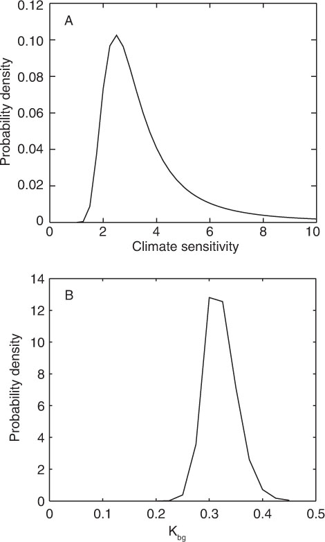
We calculated a PDF for ocean diffusivity using the statistical method described in Goes et al. (2010). Goes et al. (2010) used three globally horizontally averaged vertical tracer distributions to calculate a range of PDFs for K _bg, taking into account spatial autocorrelations as well as cross-tracer correlations of the residuals (differences between model and observations). In the current study, we use only ocean temperatures averaged from 1950 to 2000 as the observational constraint (World Ocean Atlas 2005 data downloaded from ftp.nodc.noaa.gov/pub/data.nodc/woa/WOA05nc). Other differences from Goes et al. (2010) are the use of unequally spaced model levels instead of depth as the vertical coordinate, no (globally constant) bias term in the error model and linear interpolation of model results on a finer and regularly spaced K _bg grid. The method estimates two uncertain statistical parameters endogenously in addition to K _bg. The resulting PDF of the standard deviation of the residuals has its peak at 0.6 ± 0.3 K, and the PDF of the correlation length scale of the residuals has its peak at 2.4 ± 0.2 model levels. Residuals of the low K _bg models lead to deep ocean temperatures, which are up to 2.5 K colder than the observations, whereas high K _bg models simulate a warm bias of up to 1.5 K in the thermocline (not shown).

These biases, together with the estimated standard deviation of the residuals and spatial autocorrelation, lead to probability densities of essentially zero for all values of K _bg outside the interval 0.25–0.4 (Fig. 1B). Note that this PDF is different from those of Goes et al. (2010), which in addition to the differences in the statistical method outlined above were constructed using a different version of the UVic model with elevated K _bg in the Southern Ocean.

3. Results

Results of the historical simulations with increasing K _bg lead to increased heat (Fig. 2A) and carbon (Fig. 2B) uptake due to enhanced mixing of heat and carbon into the deep ocean. As a consequence, higher ocean diffusivity result in decreased atmospheric warming; conversely, a lower K _bg leads to reduced ocean heat and carbon uptake, and increased atmospheric warming (Fig. 2C). In these simulations, CO₂ concentrations are fixed for the historical portion of the simulation, though, in the twenty-first century portion of the simulations (discussed below), atmospheric CO₂ is allowed to evolve freely in response to specified CO₂ emissions and simulated carbon sinks. In this case, increased ocean diffusivity results in a drawdown of atmospheric CO₂, contributing to an additional decreased warming of the atmosphere above that caused by enhanced heat uptake. In general, both effects of ocean carbon content and heat uptake act in the same direction, higher (lower) K _bg leads to increased (decreased) ocean heat and carbon uptake and thus less (more) atmospheric warming (see also Schmittner et al., 2009).

Fig. 2. 

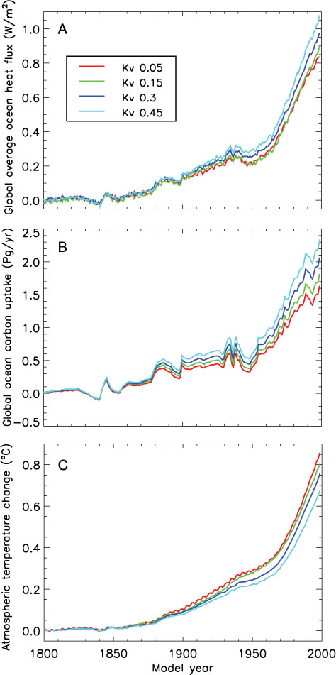
Figure 3 shows the temperature change for the twenty-first century for each of the seven different climate sensitivities, which were applied to the four different K _bg versions of the model. In all cases, the magnitude of temperature changes increased with increasing climate sensitivity, in addition to with decreasing K _bg values. At a given climate sensitivity, the effect on temperature change of increasing K _bg was equivalent to the historical portions of the simulations, although in this case, the effect of enhanced heat uptake on atmospheric temperature was amplified by a drawdown of atmospheric CO₂. For example, for a C.S. of 3.5 °C, a K _bg value of 0.05 resulted in a temperature change in 2100 of approximately 3.54 °C, while at K _bg values of 0.15, 0.3 and 0.45, temperature changes decreased progressively to 3.3, 3.2 and 3.0 °C, respectively. More interestingly, the effect of changing K _bg was not constant at all values of climate sensitivity. At lower climate sensitivities, varying K _bg had relatively little effect, whereas at higher C.S. its influence was much larger. This can be explained by the significantly higher vertical temperature gradient in the ocean in the higher C.S. simulations caused by more surface warming. The resulting increased density stratification leads to diminished exchange (mixing and overturning) between the surface and the deep ocean and hence slower uptake of anthropogenic carbon and heat by the deep ocean, which in turn causes faster warming of the surface ocean and atmosphere. In the lower C.S. simulations, on the other hand, vertical exchange in the ocean is reduced less, thus resulting in much smaller differences in atmospheric temperature change between the varying K _bg simulations.

Fig. 3. 

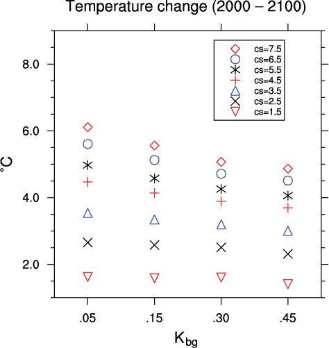
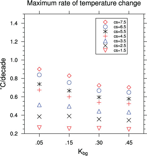
Figure 4 shows maximum decadal rates of temperature change during the twenty-first century for each combination of climate sensitivity and K _bg. At K _bg=0.05, the maximum rate of temperature change varied from 0.27 to 0.92 °C/decade for the lowest and highest climate sensitivities, respectively. These ranges decreased as a function of increasing K _bg: from 0.26 to 0.84 °C/decade for K _bg=0.15; from 0.26 to 0.74 °C/decade for K _bg=0.3; and from 0.25 to 0.73 °C/decade for K _bg=0.45. Here, we can see the non-linear interaction of climate sensitivity and ocean diffusivity more clearly. All four ocean diffusivities show very similar maximum rates of warming at the lower end of C.S. values but vary considerably at the higher end.

Fig. 4. 

By assigning probabilities to the maximum rates of temperature change using the C.S. PDF shown in Fig. 1, we can obtain PDFs for the rate of temperature change in response to A2 CO₂ emissions at a given ocean mixing rate (Fig. 5). In Fig. 5A, we can see that the most likely maximum rates of temperature change are 0.35, 0.36, 0.39 and 0.41 °C/decade for K _bg 0.45, 0.3, 0.05 and 0.15, respectively.

Fig. 5. 

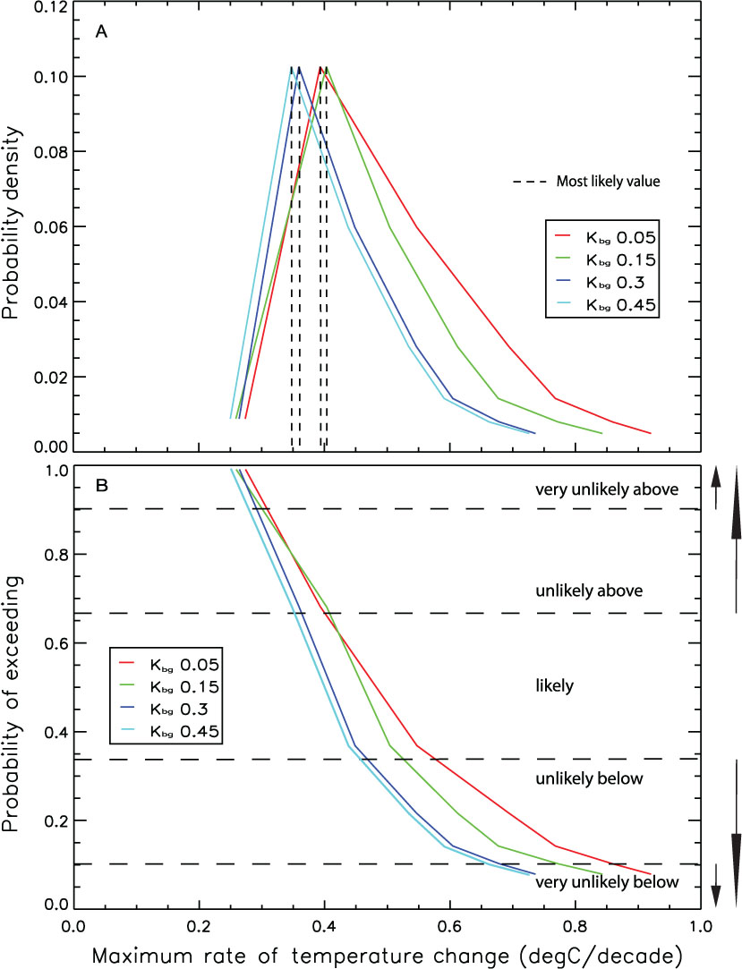
Figure 5B shows the cumulative probability distribution for each of the PDFs in Fig. 5A, which represents the probability of exceeding a given maximum rate of temperature change (°C/decade). For example, there was a 92.5% probability of exceeding 0.3°C/decade at K _bg=0.05. For the same rate of temperature change, the exceedance probability decreased to 90, 87.5 and 83% for K _bg=0.15, 0.3 and 0.45, respectively. Likely rates of temperature change were in the range of 0.36–0.47 °C/decade for K _bg=0.3 and between 0.35 and 0.46 °C/decade for K _bg=0.45. As the diffusivity rate decreased (K _bg=0.15 and 0.05), the likely ranges of maximum rate of temperature change shifted towards higher values: between 0.41 and 0.53 °C/decade for K _bg=0.15 and between 0.40 and 0.58 °C/decade for K _bg=0.05.

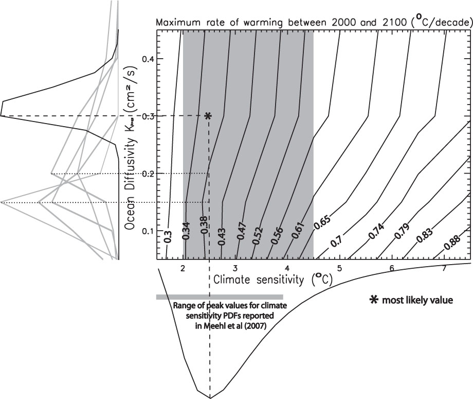
Figure 6 shows the maximum rates of temperature change between 2000 and 2100 in °C/decade as a function of both ocean diffusivity (K _bg) and C.S. (contour lines), combined with PDFs of ocean diffusivity and climate sensitivity shown in Fig. 1 (lines to the left and below the main plot). The most likely maximum rate of warming value (marked by a star in Fig. 6) was 0.36 °C/decade, corresponding to the peak of both the climate sensitivity and ocean diffusivity distribution. The shaded region indicates the likely range of warming rates, based on the climate sensitivity distribution. For comparison with previous studies, we have overlaid the K _bg PDFs from Goes et al. (2010), who calculated a range of PDFs using a combination of temperature, CFCs and C¹⁴ observations and a different version of the UVic model (grey lines on vertical axis). These PDFs from Goes et al. (2010) tend to peak at lower values of K _bg; however, the effect on the most likely rate of warming is quite small: even with a most likely K _bg probability of 0.15, the most likely rate of warming increases from 0.36 to 0.39 (less than a 10% change). Much more important is the fairly large range of climate sensitivity distributions; the grey bar below the horizontal axis of Fig. 6 indicates the range of the most likely values of climate sensitivity reported from the range of different climate sensitivity PDFs in Meehl et al. (2007). For a K _bg of 0.3, this climate sensitivity range would result in most likely rates of warming between 0.29 and 0.5 °C/decade. Given this large uncertainty arising from climate sensitivity, and to a lesser extent from ocean diffusivity uncertainty, we conclude that in general, the lower rates of warming (in the range of 0.3–0.5 °C/decade) are the most probable, whereas rates of temperature change above 0.6 °C/decade are increasingly unlikely.

Fig. 6. 

4. Discussion and conclusions

In this study, we have shown that varying C.S. and ocean diffusivity in an intermediate complexity climate model yields a range of different rates of temperature change of varying likelihoods of occurrence in response to business as usual future CO₂ emissions. We show that the maximum rate of warming during the twenty-first century would likely fall between 0.3 and 0.5 °C/decade, with a most likely value of 0.36 °C/decade. The rates of warming obtained at the higher end of this range represent extremely rapid climate change and could potentially cause serious environmental impacts on a global scale.

One potential consequence of rapid climate change is on the strength of the Atlantic Ocean meridional overturning circulation. In particular, some previous studies have suggested that a rate of change of greater than 0.3 °C/decade warming could lead to a shutdown in the Atlantic meridional overturning circulation (Stocker and Schmittner, 1997). In our simulations, we did see a decrease in the strength of the overturning circulation over the twenty-first century associated with increasing rates of temperature change, indicating that the threshold is model dependent. However, even the very high rates of change at the upper end of climate sensitivity were not sufficient to induce a complete circulation shutdown. Note, however, that our model does not include the effect of melting of the Greenland ice sheet, which would increase the probability of a future shutdown of the overturning (Swingedouw et al., 2006; Hu et al., 2011).

The impact of different rates of temperature change was an important focus of another study, by O'Neill and Oppenheimer (2004), who assessed how the potential for dangerous climate impacts may change depending on the various pathways to greenhouse gas stabilisation. The authors defined three different pathways, which are labelled as slow change, rapid change and overshoot. The slow change pathway led to medium rates of warming that slowly declined over time from an initial rate of 0.16 °C/decade. However, the rapid change simulation, with stabilisation at 600 ppm, showed a median rate of change that peaked at 0.29 °C/decade. Their overshoot simulation led to substantial additional warming that ranged from 0.1 to 0.6 °C/decade. By comparison, our results show similar rates of warming that range from 0.26 to 0.92 °C/decade, albeit with a business-as-usual, rather than a CO₂ stabilisation scenario. O'Neill and Oppenheimer (2004) emphasise that differences in transient rates of warming could significantly impact global ecosystems, and sustained rates of warming greater than 0.1 °C per decade could potentially exceed the adaptive capacity of some sensitive ecosystems.

As acknowledged by the language of the UN Framework Convention on Climate Change (UNFCCC, 1992), many environmental systems as well as the adaptive capacity of species may be vulnerable to high rates of climate change. Leemans and Eickhout (2004) used rates of temperature change to analyse global ecosystem shifts and impacts. They found that for a rate of warming of 0.1 °C/decade, 50% of all impacted ecosystems were able to adapt within a century but only 36% of all impacted forests could adapt. As the rate of change increased, the adaptive capacity of ecosystems rapidly decreased. For rates of temperature change of 0.3 °C/decade, only 30% of all impacted ecosystems and only 17% of forests could adapt naturally. According to our analysis (Fig. 5B), the rates of change greater than 0.3 °C/decade occurred with a probability of close to 90% for all configurations of ocean diffusivity. Furthermore, incorporating both climate sensitivity and ocean diffusivity likelihoods shows that the most likely maximum rates of change under the emissions scenario considered here exceed 0.3 °C/decade.

Our findings are generally consistent with those of Collins et al. (2007), who found that ocean physics perturbations do affect the rate of climate change over the twenty-first century, though to a lesser extent than do perturbations to atmospheric physics. The effect of changes in ocean diffusivity in the UVic ESCM is slightly larger than that found by Collins et al. (2007), owing to the effect of ocean diffusivity change on both heat and carbon uptake in our model. In our study, we have shown that the effect of increasing K _bg on heat uptake is amplified by increased carbon uptake, leading to an overall increased model sensitivity to K _bg changes (Schmittner et al., 2009). By contrast, Collins et al. (2007) did not include the effect of changing ocean carbon uptake on atmospheric CO₂ concentrations, which likely would have also increased the effect of ocean diffusivity changes on the rate of climate warming in their study. In addition, we have shown here that changing ocean diffusivity has a much larger effect on the rate of transient climate change for high values of climate sensitivity, compared to when climate sensitivity was low. For example, increasing K _bg from 0.05 to 0.45 decreased the maximum rate of warming by about 10% at a climate sensitivity of 2.5 °C, but by almost 25% for a climate sensitivity of 6.5 °C.

We note also that the PDF for the ocean background diapycnal diffusivity (K _bg) calculated here differs from the ones in Schmittner et al. (2009) and Goes et al. (2010). In the current analysis, we have used version 2.9 of the UVic ESCM, which includes several parameter adjustments compared to version 2.8 used by previous studies; notably, the version of the model used here does not use elevated K _bg in the Southern Ocean. Goes et al. (2010) have shown that elevated K _bg in the Southern Ocean improves ocean tracer distributions and leads to generally sharper PDFs of K _bg over the rest of the ocean, which are shifted towards lower values and appear to rule out high diffusivities (Schmittner et al., 2009; Goes et al., 2010). By contrast, our analysis resulted in higher probabilities for higher values of K _bg. However, this difference in the PDF for K _bg does not have a large bearing on the probabilities for rates of warming calculated here, as the simulated rates of warming are generally less sensitive to increases in K _bg beyond 0.3, compared to the range of K _bg between 0.1 and 0.3. Nevertheless, this does emphasise the importance of better constraining the rate of ocean mixing in order to improve predictions of future rates of climate warming.